Today, we're going to continue our walkthrough of Sample 4: Cross Validation for Regression: Auto Imports Dataset. In the previous posts, we walked through the
Initial Data Load, Imputation,
Ordinary Least Squares Linear Regression,
Online Gradient Descent Linear Regression,
Boosted Decision Tree Regression,
Poisson Regression and
Model Evaluation phases of the experiment. We also discussed
Normalization.
 |
| Experiment So Far |
Let's refresh our memory on the data set.
 |
| Automobile Price Data (Clean) 1 |
 |
| Automobile Price Data (Clean) 2 |
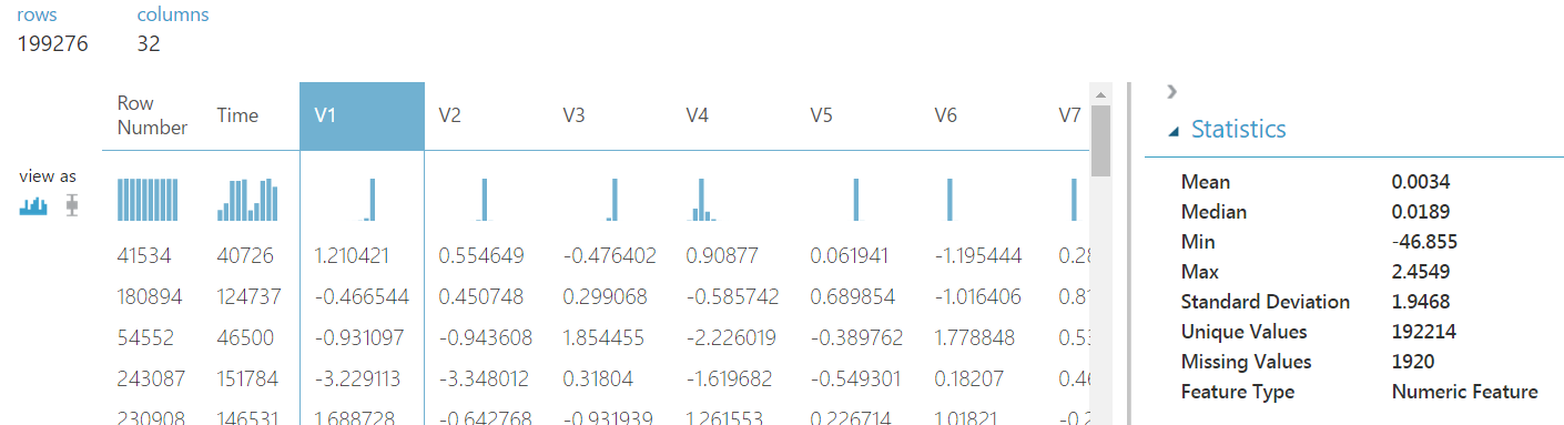
We can see that this data set contains a bunch of text and numeric data about each vehicle, as well as its price. The goal of this experiment is to attempt to predict the price of the car based on these factors.
To finish this experiment, let's take a look at Cross-Validation. We briefly touched on this topic in a previous
post as it relates to Classification models. Let's dig a little deeper into it.
As we've mentioned before, it is extremely important to have a separation between Training data (data used to train the model) and Testing data (data used to evaluate the model). This separation is necessary because it allows us to determine how well our model could predict "new" data. In this case, "new" data is data that the model has not seen before. If we were to train the model using a data set, then evaluate the model using the same data set, we would have no way to determine whether they model is good at fitting "new" data or only good at fitting data it has already seen.
In practice, these data sets are often created by cleaning and preparing a single data set that contains all of the variables needed for modelling, as well as a column or columns containing the results we are trying to predict. Then, this data is split into two data sets. This process is generally random, with a larger portion of the data going to the training set than to the testing set. However, this methodology has a major flaw. How do we know if we got a bad sample? What if by random chance, our training data was missing a significant pattern that existed in our testing set, or vice-versa? This could cause us to inappropriately identify our model as "good" due to something that is entirely outside of our control. This is where Cross-Validation comes into play.
Cross-Validation is a process for creating multiple sets of testing and training sets, using the same set of data. Imagine that we split our data in half. For the first model, we train the model using the first half of the data, then we test the model using the second half of the data. Turns out that we can repeat this process by swapping the testing and training sets. So, we can train the second model using the second half of the data, then test the model using the first half of the data. Now, we have two models trained with different training sets and tested with different testing sets. Since the two testing sets did not contain any of the same elements, we can combine the scored results together to create a master set of scored data. This master set of scored data will have a score for every record in our original data set, without ever having a single model score a record that it was trained with. This greatly reduces the chances of getting a bad sample because we are effectively scoring every element in our data, not just a small portion.
Let's expand this method a little. First, we need to break our data into three sets. The first model is trained using sets 1 and 2, and tested using set 3. The second model is trained using sets 1 and 3, and tested using set 2. The third model is trained using sets 2 and 3, and tested using set 1. In practice, the sets are known as "folds". As you can see, we can extend this method out as far as we would like to create a master set of predictions.
 |
| K Fold Cross-Validation |
There's even a subset of Cross-Validation known as "Leave One Out" where you train the model using all but one record, then score that individual record using the trained model. This process is obviously repeated for every record in the data set.
Now, the question becomes "How many folds should I have? 5? 10? 20? 1000?" This is a major question that some data scientists spend quite a bit of time working with. Fortunately for us, Azure ML automatically uses 10 folds, so we don't have to worry too much about this question. Let's see it in action.
If we look back at our previous
post, we can see that the normalization did not improve any of our models. So, for simplicity, let's remove normalization.
 |
| Experiment So Far (No Normalization) |
Now, let's take a look at the Cross Validate Model module.
 |
| Cross Validate Model |
We see that this module takes an untrained model and a data set. It also requires us to choose which column we would like to predict, "Price" in our case. This module outputs a set of scored data, which looks identical to the scored data we get from the Score Data module, although it contains all of the records, not just those in the testing set. It also outputs a set of Evaluation Results by Fold.
 |
| Evaluation Results by Fold |
This output shows a record for every fold in our Cross-Validation. Since there were ten folds, we have ten rows, plus additional rows for the mean (average) and standard deviation of each column. The columns in these results show some basic summary statistics for each fold. This data leans more heavily towards experienced data scientists. However, it can be easily used to recognize if a particular fold is strikingly different from the others. This could be helpful for determining whether there are subsets within our data that may contain completely different patterns than the rest of the data.
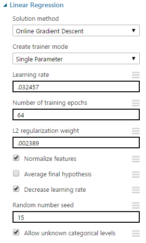
Next, we have to consider which model to input into the Cross-Validation. The issue here is that the Cross Validate Model module requires an untrained data set, while the Tune Model Hyperparameters module outputs a trained data set. So, in order to use our tuned models from the previous posts, we'll need to manually copy the tuned parameters from the Tune Model Hyperparameters module into the untrained model modules.
 |
| Online Gradient Descent Linear Regression Tuned Parameters |
 |
| Online Gradient Descent Linear Regression |
Next, we need to determine which models we want to compare. While it may be mildly interesting to compare the linear regression model trained with the 70/30 split to the linear regression model trained with Cross-Validation, that would be more of an example of the effect that Cross-Validation can have on the results. This doesn't have much business value. Instead, let's compare the results of the Cross-Validation models to see which model is best. Remember, the entire reason that we used Cross-Validation was to minimize the impact that a bad sample could have on our models. In the previous
post, we found that the Poisson Regression model was the best fit.
 |
| Ordinary Least Squares Linear Regression vs Online Gradient Descent Linear Regression |
 |
| Boosted Decision Tree Regression vs. Poisson Regression |
We can see that Poisson Regression still has the highest Coefficient of Determination, meaning that we can once again determine that it is the best model. However, this leads us to another important question. Why is it important to perform Cross-Validation if it didn't change the result? The primary answer to this involves "trust". Most of what we do in the data science world involves math that most business people would see as voodoo. Therefore, one of the easiest paths to success is to gain trust, which can be found via a preponderance of evidence. The more evidence we can provide showing that our algorithm is reliable and accurate, the easier it will be us to convince other people to use it.
Hopefully, this series opened your mind as to the possibilities of Regression in Azure Machine Learning. Stay tuned for more posts. Thanks for reading. We hope you found this informative.
Brad Llewellyn
Data Scientist
Valorem
@BreakingBI
www.linkedin.com/in/bradllewellyn
llewellyn.wb@gmail.com