As we mentioned in the previous post, there are three major concepts for us to understand about Azure Databricks, Clusters, Code and Data. For this post, we're going to talk about the interactive way to develop code, Notebooks. Azure Databricks Notebooks are similar to other notebook technologies such as Jupyter and Zeppelin, in that they are a place of us to execute snippets of code and see the results within a single interface.
 |
| Sample Notebook |
 |
| New Notebook |
 |
| Create Notebook |
 |
| Notebook Languages |
Before we get to the actually coding, we need to attach our new notebook to an existing cluster. As we said, Notebooks are nothing more than an interface for interactive code. The processing is all done on the underlying cluster.
 |
| Detached Notebook |
 |
| Attach Notebook |
 |
| Attached Notebook |
 |
| Python |
%python
import pandas as pd
pysamp = pd.DataFrame([1,2,3,4], columns=['Samp'])
display(pysamp)
<CODE END>
<CODE START>
 |
| R |
%r
rsamp <- data.frame(Samp = c(1,2,3,4))
display(rsamp)
<CODE END>
<CODE START>
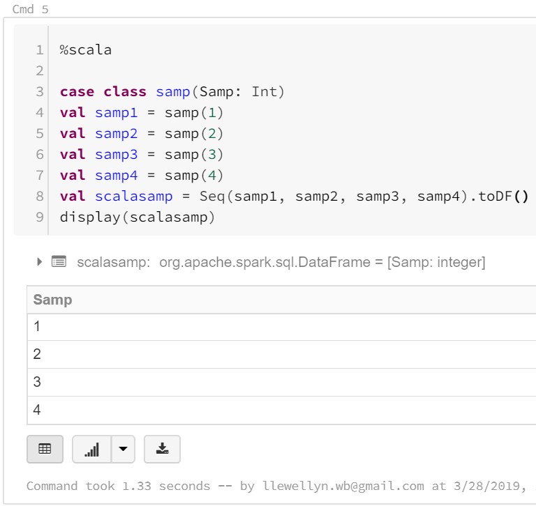 |
| Scala |
%scala
case class samp(Samp: Int)
val samp1 = samp(1)
val samp2 = samp(2)
val samp3 = samp(3)
val samp4 = samp(4)
val scalasamp = Seq(samp1, samp2, samp3, samp4).toDF()
display(scalasamp)
<CODE END>
 |
| SQL |
<CODE START>
%sql
DROP TABLE IF EXISTS sqlsamp;
CREATE TABLE sqlsamp AS
SELECT 1 AS Samp
UNION ALL
SELECT 2 AS Samp
UNION ALL
SELECT 3 AS Samp
UNION ALL
SELECT 4 AS Samp;
SELECT * FROM sqlsamp;
DROP TABLE IF EXISTS sqlsamp;
CREATE TABLE sqlsamp AS
SELECT 1 AS Samp
UNION ALL
SELECT 2 AS Samp
UNION ALL
SELECT 3 AS Samp
UNION ALL
SELECT 4 AS Samp;
SELECT * FROM sqlsamp;
<CODE END>
We can see that it's quite easy to swap from language to language within a single notebook. Moving data from one language to another is not quite as simple, but that will have to wait for another post. One interesting thing to point out is that the "%python" command is unnecessary because we chose Python as our default language when we created the Notebook.
 |
| Databricks Notebooks |
 |
| Bar Chart |
 |
| Area Chart |
 |
| Pie Chart |
 |
| Quantile Plot |
 |
| Histogram |
 |
| Box Plot |
 |
| Q-Q Plot |
We've mentioned that there are four languages that can all be used within a single notebook. There are also three additional languages that can be used for purposes other than data manipulation.
 |
| Formatted Markdown |
 |
| Markdown Code |
%md
# HEADER
## Subheader
Text
<CODE END>
We can create formatted text using Markdown. Markdown is a fantastic language for creating a rich text and image experience. Notebooks are great for sharing your work due to the fact that we can see all the code and results in a single pane. Markdown extends this even further by allow us to have rich comments along side our code as well, even including pictures and hyperlinks. You can read more about Markdown here.
 |
| LS |
%fs
ls /
<CODE END>
We also have the ability to run file system commands against the Databricks File System (DBFS). Any time we upload files to the Databricks workspace, it is stored in DBFS. We will talk more about DBFS in the next post. You can read more about DBFS here. You can read more about file system commands here.
 |
| Shell |
%sh
ls /
<CODE END>
We also have the ability to run Shell commands against the Databricks cluster. This can be very useful for performing administrative tasks. You can read more about Shell commands here.
 |
| Run |
%run ./Notebooks_Run
<CODE END>
Finally, we have the ability to run other notebooks. We simply need to give it the path to the other notebook. This will make more sense when we discuss DBFS in the next post. The "%run" command is a little different because it only allows use to provide one piece of information, the location of the notebook to run. If we were to put additional commands in this block, it would error.
All of the "%" commands we've looked at throughout this post are known as "magic commands". You can read more about magic commands here. We see that they have the amazing ability to let us use the best language for the job, depending on the task at hand. We hope this post opened your eyes to the awesome power of Notebooks. They are undoubtedly the future of analytics. The official Azure Databricks Notebooks documentation can be found here. Stay tuned for the next post where we'll dive into DBFS. Thanks for reading. We hope you found this informative.
Brad Llewellyn
Service Engineer - FastTrack for Azure
Microsoft
@BreakingBI
www.linkedin.com/in/bradllewellyn
llewellyn.wb@gmail.com