Today, we're going to talk about the Hive Database in Azure Databricks. If you haven't read the previous posts in this series, Introduction, Cluster Creation, Notebooks and Databricks File System (DBFS), they may provide some useful context. You can find the files from this post in our GitHub Repository. Let's move on to the core of this post, Hive.
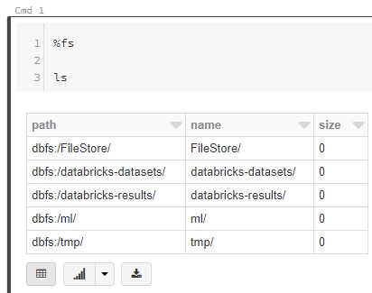
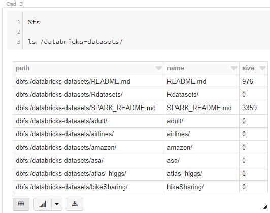
In the previous post, we looked at the way to store files, unstructured and semi-structured data in DBFS. Now, let's look at how to store structured data in a SQL format.
Each Databricks Workspace comes with a Hive Metastore automatically included. This provides us the ability to create Databases and Tables across any of the associated clusters and notebooks. Let's start by creating and populating a simple table using SQL.
 |
| Simple Table from SQL |
<CODE START>
%sql
DROP TABLE IF EXISTS Samp;
CREATE TABLE Samp AS
SELECT 1 AS Col
UNION ALL
SELECT 2 AS Col;
SELECT * FROM Samp
<CODE END>
We see that there was no configuration necessary to be able to create a SQL table in the Notebook. Now that this table is created, we can query it from a different notebook connected to a different cluster, as long as they are within the same Workspace.
 |
| Different Notebook and Cluster |
<CODE START>
%sql
SELECT * FROM Samp
<CODE END>
We're not just limited to creating tables using SQL. We can also create tables using Python, R and Scala as well.
 |
| Simple Table from Python |
<CODE START>
%python
from pyspark.sql import Row
pysamp = spark.createDataFrame([Row(Col=1),Row(Col=2)])
pysamp.write.saveAsTable('PySamp')
<CODE END>
<CODE START>
%sql
SELECT * FROM PySamp
<CODE END>
 |
| Simple Table from R |
<CODE START>
%r
library(SparkR)
rsamp <- createDataFrame(data.frame(Col = c(1,2)))
registerTempTable(rsamp, "RSampT")
s = sql("CREATE TABLE RSamp AS SELECT * FROM RSampT")
dropTempTable("RSampT")
<CODE END>
<CODE START>
%sql
SELECT * FROM RSamp
<CODE END>
 |
| Simple Table from Scala |
<CODE START>
%scala
case class samp(Col: Int)
val samp1 = samp(1)
val samp2 = samp(2)
val scalasamp = Seq(samp1, samp2).toDF()
scalasamp.write.saveAsTable("ScalaSamp")
<CODE END>
<CODE START>
%sql
SELECT * FROM ScalaSamp
<CODE END>
Each of these three languages has a different way of creating Spark Data Frames. Once the Data Frames are created, Python and Scala both support the .write.saveAsTable() functionality to create a SQL table directly. However, R requires us to create a Temporary Table first using the registerTempTable() function, then use that to create a Persisted Table via the sql() function. This is a great segue into the next topic, Temporary Tables.
A Temporary Table, also known as a Temporary View, is similar to a table, except that it's only accessible within the Session where it was created. This allows us to use SQL tables as intermediate stores without worrying about what else is running in other clusters, notebooks or jobs. Since Temporary Views share the same namespace as Persisted Tables, it's advisable to ensure that they have unique names across the entire workspace. Let's take a look.
 |
| Temporary View from SQL |
<CODE START>
%sql
DROP TABLE IF EXISTS Tempo;
CREATE TEMPORARY VIEW Tempo AS
SELECT 1 AS Col
UNION ALL
SELECT 2 AS Col;
SELECT * FROM Tempo
<CODE END>
 |
| Same Notebook, Same Cluster |
 |
| Same Notebook, Different Cluster |
 |
| Different Notebook, Same Cluster |
<CODE START>
%sql
SELECT * FROM Tempo
<CODE END>
We see that the Temporary View is only accessible from the Session that created it. Just as before, we can create Temporary Views using Python, R and Scala as well.
<CODE START>
%python
from pyspark.sql import Row
pysamp = spark.createDataFrame([Row(Col=1),Row(Col=2)])
pysamp.createOrReplaceTempView("PyTempo")
<CODE END>
<CODE START>
%sql
SELECT * FROM PyTempo
<CODE END>
<CODE START>
%r
library(SparkR)
rsamp <- createDataFrame(data.frame(Col = c(1,2)))
registerTempTable(rsamp, "RTempo")
<CODE END>
<CODE START>
%sql
SELECT * FROM RTempo
<CODE END>
<CODE START>
%scala
case class samp(Col: Int)
val samp1 = samp(1)
val samp2 = samp(2)
val scalasamp = Seq(samp1, samp2).toDF()
scalasamp.createOrReplaceTempView("ScalaTempo")
<CODE END>
<CODE START>
%sql
SELECT * FROM ScalaTempo
<CODE END>
Again, we see the similarities between Python and Scala, with both supporting the .createOrReplaceTempView() function. R is the odd man out here using the same registerTempTable() function we saw earlier.
These are great ways to create Persisted and Temporary Tables from data that we already have access to within the notebook. However, Hive gives us access to something that is simply not possible with most other SQL technologies, External Tables.
Simply put, an External Table is a table built directly on top of a folder within a data source. This means that the data is not hidden away in some proprietary SQL format. Instead, the data is completely accessible to outside systems in its native format. The main reason for this is that it gives us the ability to create "live" queries on top of text data sources. Every time a query is executed against the table, the query is run against the live data in the folder. This means that we don't have to run ETL jobs to load data into the table. Instead, all we need to do is put the structured files in the folder and the queries will automatically surface the new data.
In the previous post, we mounted an Azure Blob Storage Container that contains a csv file. Let's build an external table on top of that location.
<CODE START>
%sql
CREATE EXTERNAL TABLE Ext (
age INT
,capitalgain INT
,capitalloss INT
,education STRING
,educationnum INT
,fnlwgt INT
,hoursperweek INT
,income STRING
,maritalstatus STRING
,nativecountry STRING
,occupation STRING
,race STRING
,relationship STRING
,sex STRING
,workclass STRING
)
LOCATION '/mnt/breakingbi/'
ROW FORMAT DELIMITED FIELDS TERMINATED BY ','
STORED AS TEXTFILE;
SELECT * FROM Ext
WHERE education != 'education'
<CODE END>
We see that it's as simple as defining the schema, location and file type. The one downside is that the current version of Azure Databricks at the time of writing does not support skipping header rows. So, we do need to add a line of logic to remove these records. Before we move on to how to hide that issue, let's look at one neat piece of functionality with External Tables. Not only do they support reading from file locations, they also support writing to file locations. Let's duplicate all of the records in this table and see what happens to the mounted location.
We see that the number of records in the table have doubled. When we look at the mounted location, we also see that there have been some new files created. In typical Spark style, these files have very long, unique names, but the External Table doesn't care about any of that.
Finally, let's look at how to clean up our external table so that it doesn't show the header rows anymore. We can do this by creating a View (not to be confused with the Temporary View we discussed earlier).
<CODE START>
%sql
CREATE VIEW IF NOT EXISTS vExt AS
SELECT * FROM Ext
WHERE education != 'education';
SELECT * FROM vExt
<CODE END>
A View is nothing more than a canned SELECT query that can be queried as if it was a Table. Views are a fantastic way to obscure complex technical logic from end users. All they need to be able to do is query the table or view, they don't need to worry about the man behind the curtain.
We hope this post enlightened you to the powers of using SQL within Azure Databricks. While Python, R and Scala definitely have their strengths, the ability to combine those with SQL provide a level of functionality that isn't really matched by any other technology on the market today. The official Azure Databricks SQL documentation can be found here. Stay tuned for the next post where we'll dig into RDDs, Data Frames and Datasets. Thanks for reading. We hope you found this informative.
Brad Llewellyn
Service Engineer - FastTrack for Azure
Microsoft
@BreakingBI
www.linkedin.com/in/bradllewellyn
llewellyn.wb@gmail.com
 |
| Temporary View from Python |
<CODE START>
%python
from pyspark.sql import Row
pysamp = spark.createDataFrame([Row(Col=1),Row(Col=2)])
pysamp.createOrReplaceTempView("PyTempo")
<CODE END>
<CODE START>
%sql
SELECT * FROM PyTempo
<CODE END>
 |
| Temporary View from R |
<CODE START>
%r
library(SparkR)
rsamp <- createDataFrame(data.frame(Col = c(1,2)))
registerTempTable(rsamp, "RTempo")
<CODE END>
<CODE START>
%sql
SELECT * FROM RTempo
<CODE END>
 |
| Temporary View from Scala |
<CODE START>
%scala
case class samp(Col: Int)
val samp1 = samp(1)
val samp2 = samp(2)
val scalasamp = Seq(samp1, samp2).toDF()
scalasamp.createOrReplaceTempView("ScalaTempo")
<CODE END>
<CODE START>
%sql
SELECT * FROM ScalaTempo
<CODE END>
Again, we see the similarities between Python and Scala, with both supporting the .createOrReplaceTempView() function. R is the odd man out here using the same registerTempTable() function we saw earlier.
These are great ways to create Persisted and Temporary Tables from data that we already have access to within the notebook. However, Hive gives us access to something that is simply not possible with most other SQL technologies, External Tables.
Simply put, an External Table is a table built directly on top of a folder within a data source. This means that the data is not hidden away in some proprietary SQL format. Instead, the data is completely accessible to outside systems in its native format. The main reason for this is that it gives us the ability to create "live" queries on top of text data sources. Every time a query is executed against the table, the query is run against the live data in the folder. This means that we don't have to run ETL jobs to load data into the table. Instead, all we need to do is put the structured files in the folder and the queries will automatically surface the new data.
In the previous post, we mounted an Azure Blob Storage Container that contains a csv file. Let's build an external table on top of that location.
 |
| Create External Table |
<CODE START>
%sql
CREATE EXTERNAL TABLE Ext (
age INT
,capitalgain INT
,capitalloss INT
,education STRING
,educationnum INT
,fnlwgt INT
,hoursperweek INT
,income STRING
,maritalstatus STRING
,nativecountry STRING
,occupation STRING
,race STRING
,relationship STRING
,sex STRING
,workclass STRING
)
LOCATION '/mnt/breakingbi/'
ROW FORMAT DELIMITED FIELDS TERMINATED BY ','
STORED AS TEXTFILE;
SELECT * FROM Ext
WHERE education != 'education'
<CODE END>
We see that it's as simple as defining the schema, location and file type. The one downside is that the current version of Azure Databricks at the time of writing does not support skipping header rows. So, we do need to add a line of logic to remove these records. Before we move on to how to hide that issue, let's look at one neat piece of functionality with External Tables. Not only do they support reading from file locations, they also support writing to file locations. Let's duplicate all of the records in this table and see what happens to the mounted location.
 |
| Insert Into External Table |
 |
| Mounted Location Post-Insert |
Finally, let's look at how to clean up our external table so that it doesn't show the header rows anymore. We can do this by creating a View (not to be confused with the Temporary View we discussed earlier).
 |
| Create View |
<CODE START>
%sql
CREATE VIEW IF NOT EXISTS vExt AS
SELECT * FROM Ext
WHERE education != 'education';
SELECT * FROM vExt
<CODE END>
A View is nothing more than a canned SELECT query that can be queried as if it was a Table. Views are a fantastic way to obscure complex technical logic from end users. All they need to be able to do is query the table or view, they don't need to worry about the man behind the curtain.
We hope this post enlightened you to the powers of using SQL within Azure Databricks. While Python, R and Scala definitely have their strengths, the ability to combine those with SQL provide a level of functionality that isn't really matched by any other technology on the market today. The official Azure Databricks SQL documentation can be found here. Stay tuned for the next post where we'll dig into RDDs, Data Frames and Datasets. Thanks for reading. We hope you found this informative.
Brad Llewellyn
Service Engineer - FastTrack for Azure
Microsoft
@BreakingBI
www.linkedin.com/in/bradllewellyn
llewellyn.wb@gmail.com