Monday, October 27, 2014

Data Mining in Excel Part 26: Neural Networks

Today, we'll be talking about the final classification algorithm in the Microsoft Data Mining stack, Neural Networks.  A Neural Network is the pathways that animals (including people) use to develop thoughts and ideas.  Technically, this algorithm builds an Artificial Neural Network in an attempt to emulate that kind of behavior.  In Excel, this algorithm is only accessible through the "Add Model to Structure" button.
Add Model to Structure
If you read our post on Logistic Regression, you may recognize some of the concepts here.  The Logistic Regression algorithm is actually a special case of the Neural Network algorithm created by excluding any hidden layers.  For more information about Artificial Neural Networks, read this.  Let's get started.
Select Structure
First, we need to select the "Classify Purchased Bike" structure to store our model.
Select Algorithm
Then, we need to select the "Microsoft Neural Network" algorithm.  Let's take a look at the parameters.
Parameters
The more observant views might notice that the only difference between these parameters and the Logistic Regression parameters is the addition of Hidden Node Ratio.  This makes perfect sense because, as we said earlier, the Logistic Regression algorithm is simply the Neural Network algorithm with no hidden layer, i.e. Hidden Node Ratio = 0.  The Hidden Node Ratio is most useful parameter in this algorithm and can be used to drastically change the model.  For more information about these parameters, read this.  Let's move on.
Select Columns
As usual, we want to use all of the columns except ID (_RowIndex) and Purchased Bike to predict Purchased Bike.
Create Model
Finally, we need to create the model.  Let's check out the results.
Discrimination Report
This Discrimination Report says that we should focus on customers from the Pacific, have a Professional occupation, 1 car, or 3 kids.  You can keep going with that logic for as long as you need.  Just for kicks, let's see what happens if we try a couple different values for Hidden Node Ratio.
Discrimination Report (1 HNR)
This model has a Hidden Node Ratio of 1.  This model still has most of the same favorable attributes as the previous one.  That's a good thing because it implies that the model is stable, and therefore good.  Let's try a Hidden Node Ratio of 10.
Discrimination Report (10 HNR)
This model looks pretty similar to the others as well.  We should note that we can't suggest stability of the model by using the Discrimination Report.  What we really need to do is see how much the predicted values vary, or don't vary, across the models.  Even better, we could compare the predictions from the Neural Network models to the other classification models we've built previously.  However, we're not quite there yet.  Keep an eye out for our next post where we'll be talking about Accuracy Charts.  Thanks for reading.  We hope you found this informative.

P.S.

We wanted to discuss the Sequence Clustering Algorithm next.  However, we can't add a Sequence Clustering Model to a Structure without a Sequence ID, yet we can't find a way to create a Structure with a Sequence ID.  So, if you know anything about building a Sequence Clustering Model using the Excel interface, let us know in the comments.

Brad Llewellyn
Director, Consumer Sciences
Consumer Orbit
llewellyn.wb@gmail.com
http://www.linkedin.com/in/bradllewellyn

Monday, October 20, 2014

Data Mining in Excel Part 25: Naive Bayes

Today, we're going to talk another of the "hidden" algorithms in the Data Mining Add-ins for Excel, Naive Bayes.  Naive Bayes is a classification algorithm, similar to Decision Trees and Logistic Regression, that attempts to predict categorical values.  A special catch of this procedure is that it can only use discrete and discretized values, meaning continuous values like Age and Income cannot be used.  If you want to use these types of values, then you would need to discretize them first.  To read more about Naive Bayes, navigate here.  In order to use this algorithm, we need to add another model to our existing structures using the "Add Model to Structure" button.
Add Model to Structure
Let's get started.
Select Algorithm
First, we need to select the Naive Bayes algorithm.  Before we move on, let's take a look at the Parameters.
Parameters
Just like that with Logistic Regression, this algorithm have very few parameters.  In fact, the only parameter that actually affects the model is the Minimum Dependency Probability.  Altering this value will increase or decrease the number of predictors in the model.  For more information on these parameters, read this.  Let's move on.
Select Columns
Since the structure has defined Age and Income as Continuous variables, this algorithm will not let us use them.  So, the only thing we need to change here is set Purchased Bike to "Predict Only".
Create Model
Finally, we create our model using the naming convention we've been following for this entire series.  It's important to note that, just like Logistic Regression, this algorithm doesn't support drillthrough.  Let's jump to the output.
Dependency Network
Well, we have an issue already.  There are no variables in the model other than Purchased Bike.  This means that we can't predict values with this model.  This is very likely due to the fact that the best predictors are discretized versions of Income and Age.  To test this, let's create another structure that discretizes those values and use that for a new model.  For more information on how to create a mining structure, read this.
Select Columns (Discretized)
Notice how Age and Income are inputs now?  That's because they're no longer Continuous variables.  Let's check out this model.
Dependency Network (Discretized)
For some reason, discretizing Age and Income cause Cars to become statistically significant.  This model is still pretty bare, let's change the parameters to get a fuller model.
Parameters (.01 MDP)
We needed to reduce the Minimum Dependency Probability all the way to .01, which is almost as low as it can be, before we actually got any change in the model.  At this point, we're thoroughly convinced that this algorithm is not appropriate for this data set.  However, we'll continue the analysis as a demonstration.  Let's check out the model.
Dependency Network  (.01 MDP)
We see that Marital Status and Cars are predictors for Purchased Bike.  Next, let's jump over to Attribute Profiles.
Attribute Profiles
We can see the breakdown of each predictor as it relates to each value of Purchased Bike.  The differences are pretty minor.  So, let's move on to the Attribute Characteristics.
Attribute Characteristics
By now, you should have noticed that this is exactly the same type of output we saw for the Clustering Algorithm, albeit less useful because of the quality of the model.  This screen shows us what makes up each individual value of Purchased Bike.  However, we find the Attribute Discrimination to be much more useful.
Attribute Discrimination
This view will show you what attributes correspond best with certain outcomes.  Not surprisingly, we see that people with no cars tend to buy bikes while people with 2 cars do not.  We also see that married people don't usually buy bikes while Single people do.

Just like with Logistic Regression, this algorithm is typically not as useful as Decision Trees.  However, it will typically perform better.  So, the goal is to see whether the increase processing and querying time for the more complex models actually yields better predictions.  In this case, the Decision Tree model is significantly better.  Keep an eye for the next post where we'll be talking about Neural Networks.  Thanks for reading.  We hope you found this informative.

Brad Llewellyn
Director, Consumer Sciences
Consumer Orbit
llewellyn.wb@gmail.com
http://www.linkedin.com/in/bradllewellyn

Monday, October 13, 2014

Data Mining in Excel Part 24: Logistic Regression

Today, we're going to start talking about the last few algorithms in the Microsoft Data Mining Stack.  These algorithms can only be accessed via the "Add Model to Structure" tool.
Add Model to Structure
Specifically, this post will be talking about the Logistic Regression algorithm.  Logistic Regression is designed to predict Binary (Yes/No, 1/0) values.  To find out more about Logistic Regression, read this.  However, Microsoft's algorithm expands the scope of the procedure to allow it predict more than just 2 values.  It is closely related to the Decision Tree algorithm, which is where we going to start.  In a previous post, we built a classification model for predicting Purchased Bike.  Let's add another model to that structure using the Logistic Regression algorithm and see what we get.
Select Structure
The first step is to select the "Classify Purchased Bike" structure.
Select Algorithm
Next, we need to select the "Microsoft Logistic Regression" algorithm.  Let's see what kind of parameters we have.
Parameters
Compared to the other algorithms, Logistic Regression has much fewer parameters.  In fact, none of the parameters alter the methodology behind how the model is built.  They all affect what data the model sees when it is being trained.  For more information on these parameters, read this.  Let's move on.
Select Columns
Now, we need to select which columns we will use for what purposes.  Since this is a simple question, we want to use every column except ID (called _RowIndex here for some reason) and Purchased Bike, to predict Purchased Bike.
Create Model
Finally, we create the model inside the existing structure.  It's interesting to note that this algorithm does not allow drillthrough.  You'll understand why as soon as you see the Browse window.
Browse
This is the only option we have for viewing this model.  Many of you may recognize this as a Discrimination Report.  This report shows us which input values seem to correspond with certain output values.  For instance, we see that people with 5 children, 4 cars, or 3 cars don't usually buy bikes.  However, the odds of selling to customers with high income or that live in the Pacific are much higher.  Obviously, there's nowhere to click here to be able to drillthrough, which is why the option was no selectable before.

Our customization options lie in the upper-right corner of the window.  Here, we can select which output variable we want to look at, assuming we have more than one, and which values within that variable we want to compare.  In our case, we had one variable with two values, so the choice is pretty simple.  We can also choose to look at a subset of our population by applying filters in the upper-left corner of the window.

You might be wondering why anyone would use this algorithm when the Decision Tree algorithm seems to be much more informative.  In fact, the Decision Tree algorithm is built with some of the same logic as the Logistic Regression algorithm, just in a more complex manner.  This is especially apparent because we don't really have any parameters to tweak this algorithm to our liking.  Well, if you were working with enormous data sets, the Decision Tree algorithm may have significant performance issues.  So, one methodology for professional data miners is to build a lot of candidate models using different parameters and different algorithms.  Then, they compare the models to see which give better results with less work.  For instance, if your Decision Tree model gives very similar predictions to your Logistic Regression model, but takes all day to run, then you should consider throwing the Decision Tree model away, or finding a combination of parameters that gives you a better prediction.  When you're dealing with enterprise-wide Data Mining operations, time is money and should be considered.  Stay tuned for our next post where we'll be talking about Naive Bayes.  Thanks for reading.  We hope you found this informative.

Brad Llewellyn
Director, Consumer Sciences
Consumer Orbit
llewellyn.wb@gmail.com
http://www.linkedin.com/in/bradllewellyn

Monday, October 6, 2014

Data Mining in Excel Part 23: Multiple Models in a Single Structure

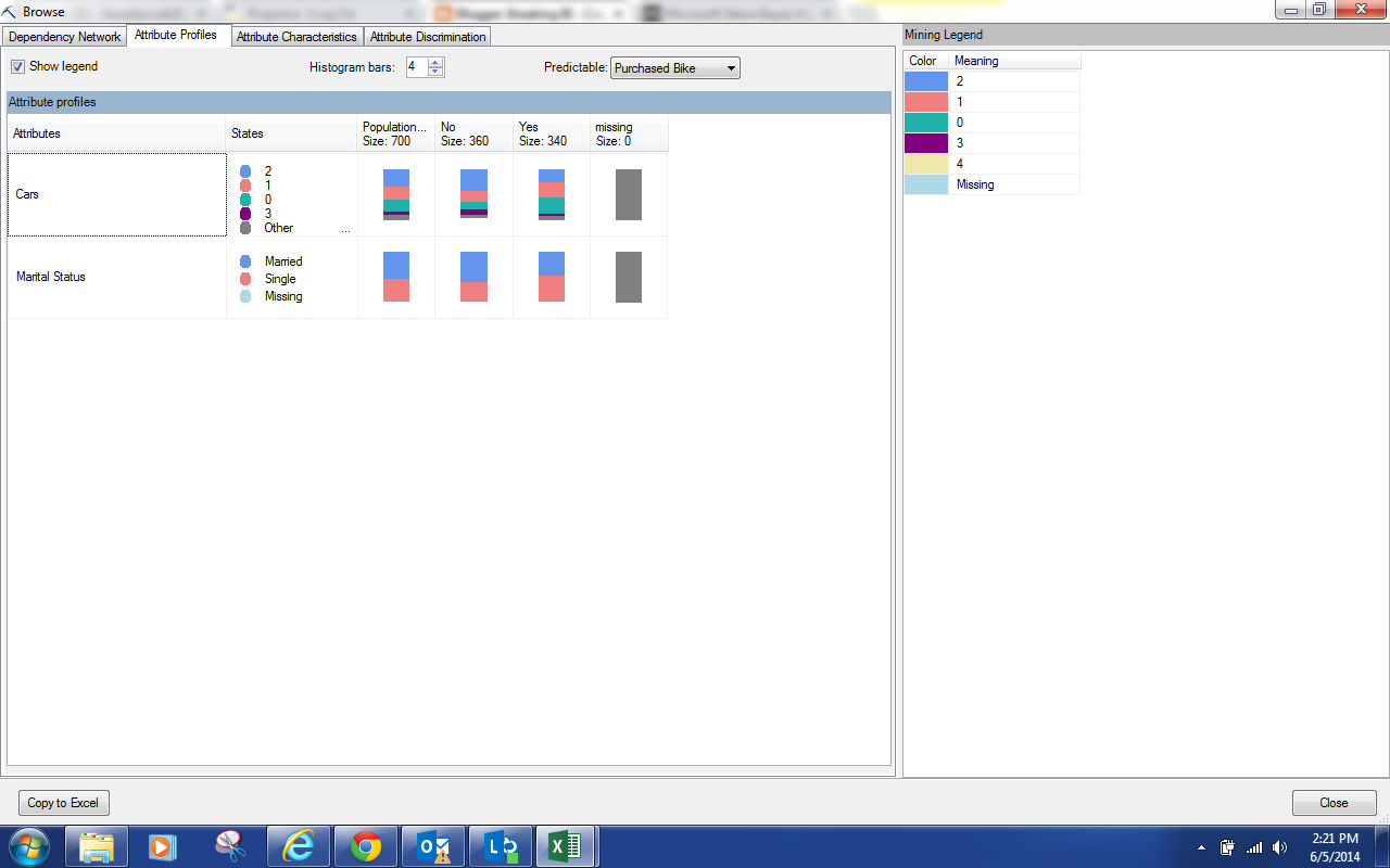
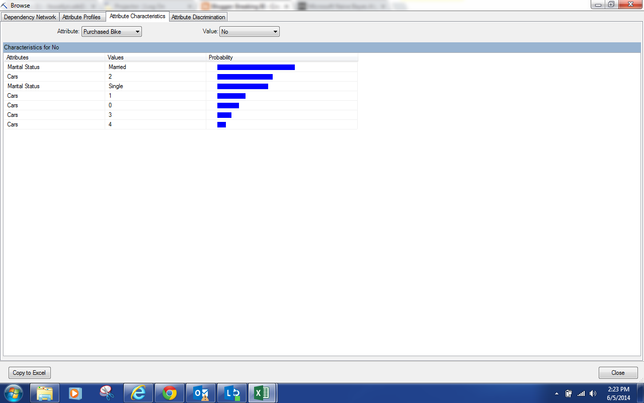
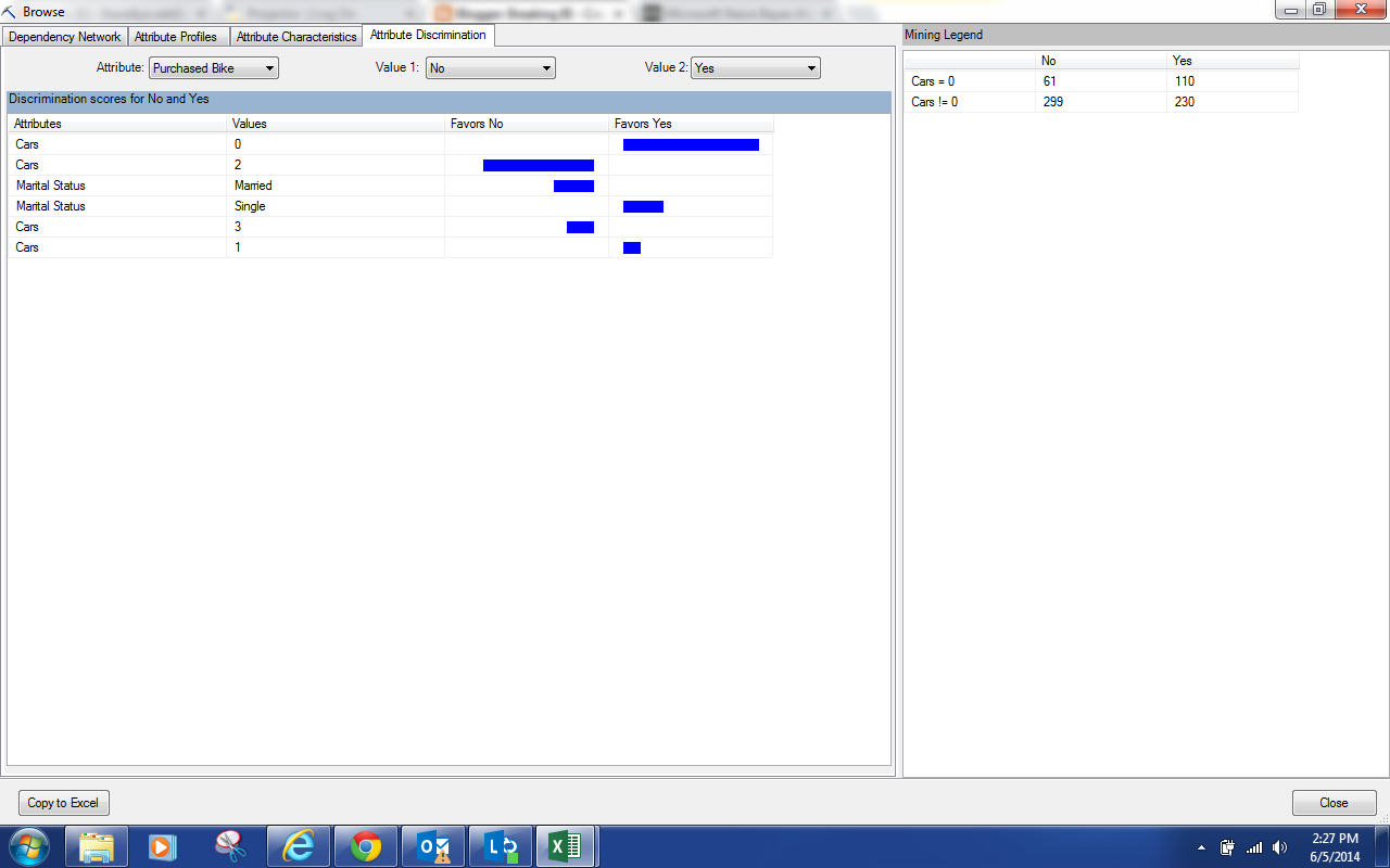
Today, we're going to get a little more into the nuts-and-bolts and talk about Mining Structures and Mining Models.  A Mining Structure is basically a table.  It has some data that you would like to do analysis on.  The first step to any analysis is deciding what type of question you want to ask.  Once you've decided the question, then you can pick your data source by creating a Mining Structure.  Now that you have a structure, you can create as many models as you need to answer your question.  Each model should be built to attempt to answer the question in a slightly different way.  For instance, if you want to predict whether a customer will buy a bike, you could create a Decision Tree Model and a Naive Bayes Model.  Then, you could compare the two models to see which one gives you the best results.

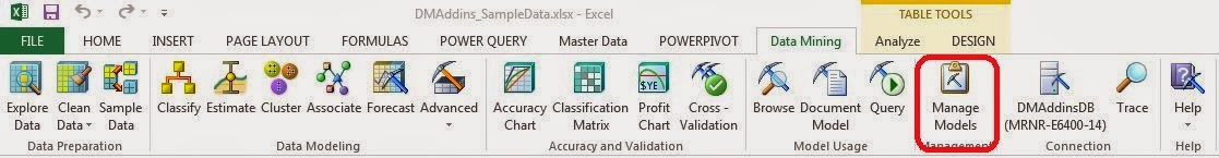
Up to now, we've been using the built-in algorithms to do our analysis.  There's nothing wrong with this.  But, it requires to create a new mining structure each time we want to run an analysis.  We can look at each of these structures using the Manage Models tool.
Manage Models
Let's see what we have.
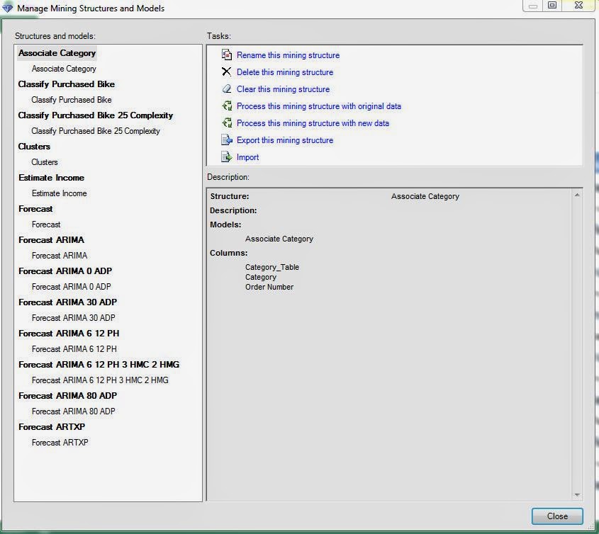
Mining Structures and Models
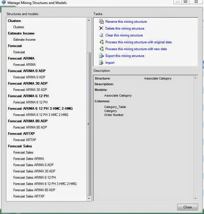
Here, we have all of the Mining Structures and Mining Models we've created so far in this blog series.  However, we don't need this many structures.  All of the Forecasting Models use the same data to answer the same question.  They could have easily been placed inside a single "Forecast" Structure for organizational purposes.  The question becomes "How do we make these Structures and Models?"
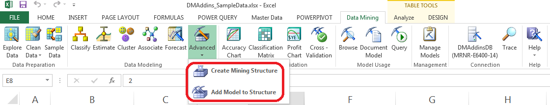
Advanced
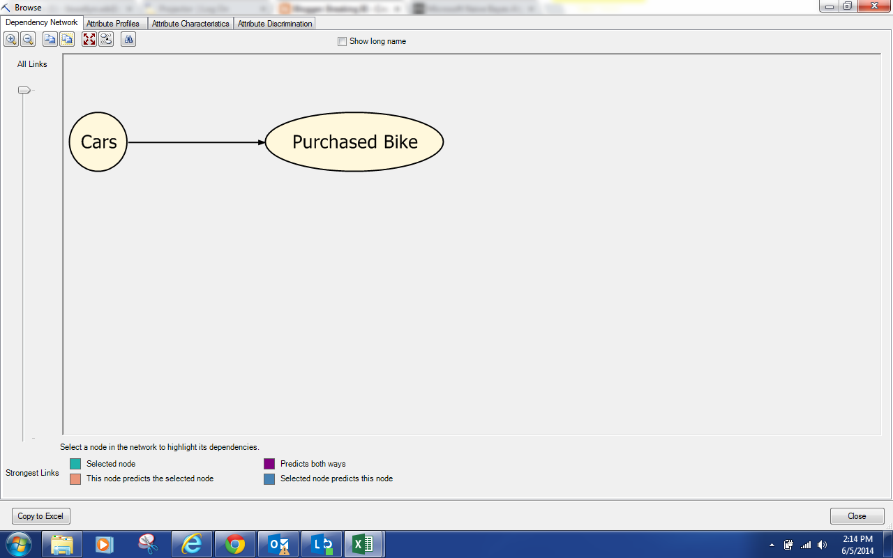
As a simple demonstration, let's take all of our Forecasting Models and put them under a single "Forecast Sales" Structure.  First, we need to create a Mining Structure with the data we would like to use for Forecasting.
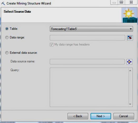
Select Data Source
Of course, the first step is to select the source of the data.  We'll be using the Monthly Sales table we used in the previous Forecasting posts.  Let's move on.
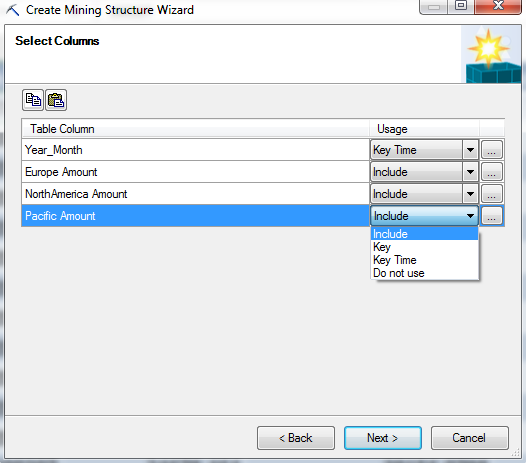
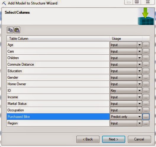
Select Columns
Here, we have to select which columns from the table we would like to use.  For each column, we have four options.  We could include the column, which allows it to be as a predictor and regressor in the models.  We could make the column a key, which means that it is a unique identifier for each row.  We could the column a key time, which is the same as a key, just for Forecasting purposes.  Lastly, we could choose to exclude the column entirely which would mean that we cannot use it in any of the models within this structure.  Also, if we click on the "..." beside any of the values, we can choose the data type and content type for that column.
Data Type
The data type of a column determines how algorithms deal with it.  For instance, a Text column is treated as a dimension or slicer, which is great for building decision trees.  A Boolean (true/false) is also great as a slicer.  Long (integer) and Double (decimal) are numeric values that can be used in almost any way you would like.  Lastly, you can choose Date which is also numeric.  This means that they can be ordered and sliced.  However, Dates cannot be used as part of an arithmetic model, such as linear regression, because you can't simply perform arithmetic between dates and numbers.
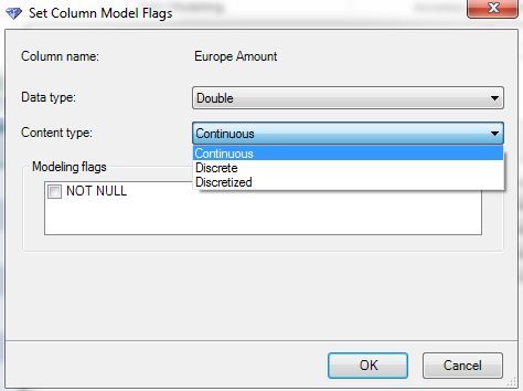
Content Types
A content type defines the way that a column is used.  A Continuous variable is treated just like a regular number.  You can add them, subtract them, etc. A discrete variable is used a slicer, such as Region = "Pacific".  The final data type is a little more complex.  Let's say you have a numeric variable that you would like to use a slicer, e.g. Age.  If you set it as discrete, it would treat each as a completely separate category.  This would lead to a LOT of possible values.  A general rule of thumb is that you don't want a discrete variable to have more than around six possible values.  So, if you set Age as Discretized, you could create "buckets" for Age.  This would effectively create another column that takes values such as "20-29", "30-39", etc.  You don't have to worry about creating these buckets yourself either.  The Data Mining tools have a built-in algorithm for discretizing data in an optimal way.  Lastly, you can set a column as NOT NULL.  This means that you will get an error if there is any null or blank value in that column.  Let's move on.
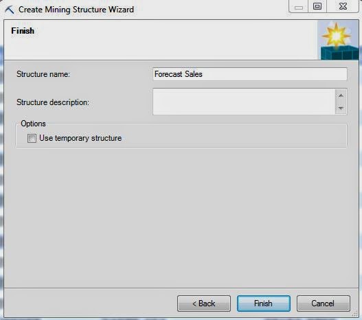
Create Structure
The final step is to give the Structure a name and create it.
Manage Models (Empty Structure)
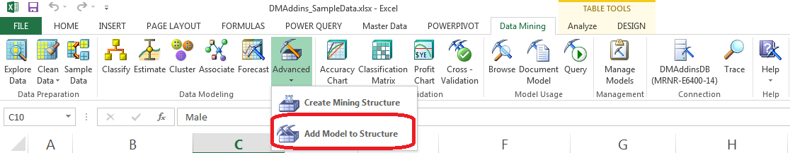
Now, we can see our empty Mining Structure at the bottom of the list.  Let's add the Forecast model to this structure using the "Add Model to Structure" button under the Advanced tool.
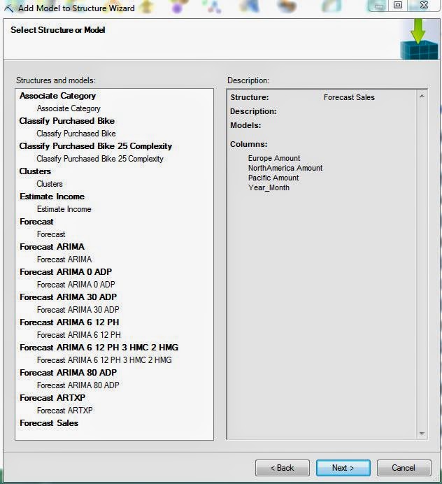
Select Structure
Since we've already stored our data within a Structure, the first step to this analysis is to select that structure.
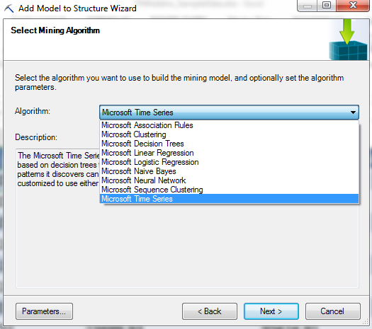
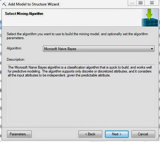
Select Algorithm
Then, we need to select the algorithm that we would like to use.  There are a few algorithms in this list that we haven't seen yet.  The only way to access "Logistic Regression", "Naive Bayes", "Neural Network", and "Sequence Clustering" within Excel is with this method.  However, the first three algorithms are actually just different methods for doing analyses we've already done.  We'll touch on them in later posts.  Sequence Clustering is something we haven't talked about yet.  Unfortunately, we won't be covering Sequence Clustering in this series.  However, you are more than welcome to tinker with it on your own.  Back on topic, we don't need any parameters for the "Forecast" model because this was the basic model.  We'll use parameters for the rest of the models.  Let's keep going.
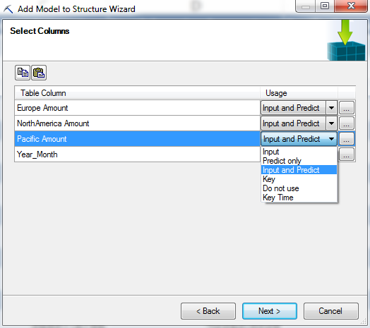
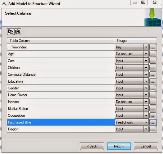
Select Columns for Algorithm
This window looks like the same window we used when we were creating the structure.  However, our options are different now.  For one, we can't change the usage for Year_Month at all.  For our model variables, we have a few options.  As you probably remember, the ARTXP model allows each series to be used to predict values for the others series as well as itself.  That means that each series is both an "Input" (used for predictions) and a "Predict" (predictions).  Let's say you don't want to predict values for Pacific, but you would still like that series to be used to predict values for North America.  In order to do that, all you have do is set Pacific to "Input".  You can also choose not to use a column at all if you wish.  Also, if we clicked on the "..." again, we would see that we no longer have the option of changing these data types.  Let's move on.
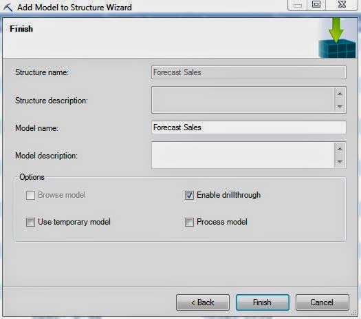
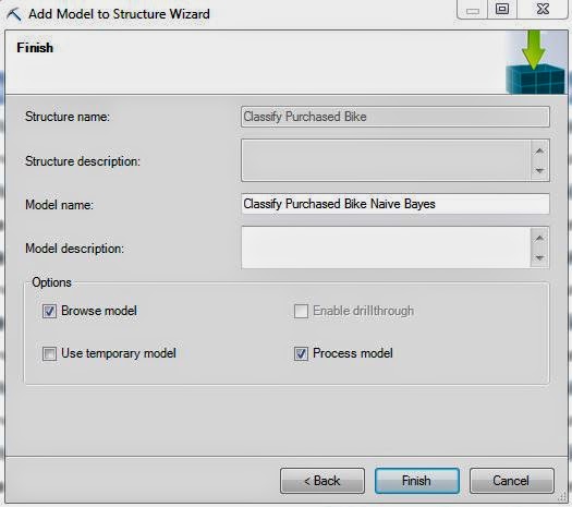
Create Model
Finally, we get to create our Mining Model.  There's another option here that we haven't seen yet, "Process Model".  Processing the model would allow us to use it immediately for our analysis.  Since we're only interested in moving the models into the structure for now, there's no reason to process the model.  We can always come back and process the model later.

Now, all we have to do is repeat this process for the rest of the models and we'll have moved all of models into a single structure.
Manage Models (Complete Structure)
Now that we're getting further along in this series, we hope that a lot of the pieces are starting to come together.  The Data Mining Add-in for Excel is extremely powerful and we hope that you'll find a use for it in your business.  Keep an eye out for our next post where we'll be talking about Logistic Regression.  Thanks for reading.  We hope you found this informative.

Brad Llewellyn
Director, Consumer Sciences
Consumer Orbit
llewellyn.wb@gmail.com
http://www.linkedin.com/in/bradllewellyn