 |
| Sample 3: Cross Validation for Binary Classification Adult Dataset |
 |
| Adult Census Income Binary Classification Dataset (Visualize) |
 |
| Adult Census Income Binary Classification Dataset (Visualize) (Income) |
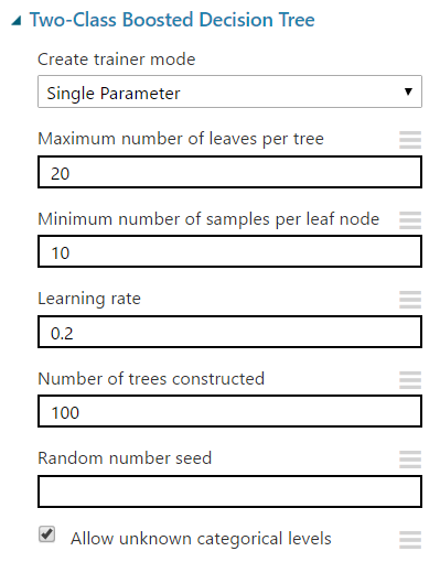 |
| Two-Class Boosted Decision Tree |
The "Maximum Number of Leaves per Tree" parameter allows us to set the number of times the tree can split. It's important to note that splits early in the tree are caused by the most significant predictors, while splits later in the tree are less significant. This means that the more leaves you have (and therefore more splits), the higher your chance of overfitting is. This is why Validation is so important.
The "Minimum Number of Samples per Leaf Node" parameters allows us to set the significance level required for a split to occur. With this value set at 10, the algorithm will only choose to split (this known as creating a "new rule") if at least 10 rows, or observations, will be affected. Increasing this value will lead to broad, stable predictions, while decreasing this value will lead to narrow, precise predictions.
The "Learning Rate" parameter allows us to set how much difference we see from tree to tree. MSDN describes this quite well as "the learning rate determines how fast or slow the learner converges on the optimal solution. If the step size is too big, you might overshoot the optimal solution. If the step size is too small, training takes longer to converge on the best solution."
Finally, this algorithm lets us select a "Create Trainer Mode". This is extremely useful if we can't decide exactly what parameters we want. We'll take more about parameter selection in a later post. If you want to learn more about this algorithm, read here and here. Let's visualize this tool.
 |
| Two-Class Boosted Decision Tree (Visualize) |
 |
| Condensed Experiment |
 |
| Train Model |
 |
| Train Model (Visualization) |
 |
| Train Model (Visualization) (Zoom) |
As you can see, each split in the tree relies on a single variable in a single expression, known as a predicate. The first predicate says
marital-status.Married-civ-spouse <= 0.5
We've talked before about the concept of Dummy Variables. When you pass a categorical variable to a numeric algorithm like this, it has to translate the values to numeric. It does this by creating Dummy, or Indicator, Variables. In this case, it created Dummy Variables for the "marital-status" variable. One of these variables is "marital-status.Married-civ-spouse". This variable takes a value of 1 if the observation has "marital-status = Married-civ-spouse" and 0 otherwise. Therefore, this predicate is really just a numeric way of saying "Does this person have a Marital Status of "Married-Civ-Spouse". We're not sure exactly what this means because this isn't our data set, but it's the most common variable in the dataset. Therefore, it probably means being married and living together.
Under the predicate definition, we also see a value for "Split Gain". This is a measure of how significant the split was. A large value means a more significant split. Since Google is our best friend, we found a very informative answer on StackOverflow explaining this. You can read it here.
What we find very interesting about this tree structure is that it is not "balanced". This means that in some cases, we can reach a prediction very quickly or very slowly depending on which side of the tree we are on. We can see one prediction in Level 2 (the root level is technically considered Level 0. This means that the 3rd level is considered Level 2). We're not sure what causes the tree to choose whether to predict or split. The MSDN article seems to imply that it's based on the combination of the "Minimum Number of Samples per Leaf Node" as well as some internal Information (or Split Gain) threshold. Perhaps one of our readers can enlighten us about this.
Since we talked heavily about Cross-Validation in the previous post, we won't go into too much detail here. However, it may be interesting to see the Contingency table to determine how well this model predicted our data.
 |
| Contingency Table (Two-Class Boosted Decision Tree) |
 |
| Contingency Table (Two-Class Averaged Perceptron) |
Brad Llewellyn
BI Engineer
Valorem Consulting
@BreakingBI
www.linkedin.com/in/bradllewellyn
llewellyn.wb@gmail.com