Today, we're going to continue looking at Sample 3: Cross Validation for Binary Classification Adult Dataset in Azure Machine Learning. In the previous posts, we looked at the
ROC,
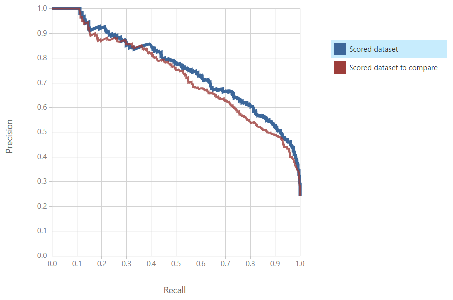
Precision/Recall and Lift tabs of the "Evaluate Model" module. In this post, we'll be finishing up Sample 3 by looking at the "Threshold" and "Evaluation" tables of the Evaluate Model visualization. Let's start by refreshing our memory on the data set.
 |
| Adult Census Income Binary Classification Dataset (Visualize) |
 |
| Adult Census Income Binary Classification Dataset (Visualize) (Income) |
This dataset contains the demographic information about a group of individuals. We see the standard information such as Race, Education, Martial Status, etc. Also, we see an "Income" variable at the end. This variable takes two values, "<=50k" and ">50k", with the majority of the observations falling into the smaller bucket. The goal of this experiment is to predict "Income" by using the other variables.
 |
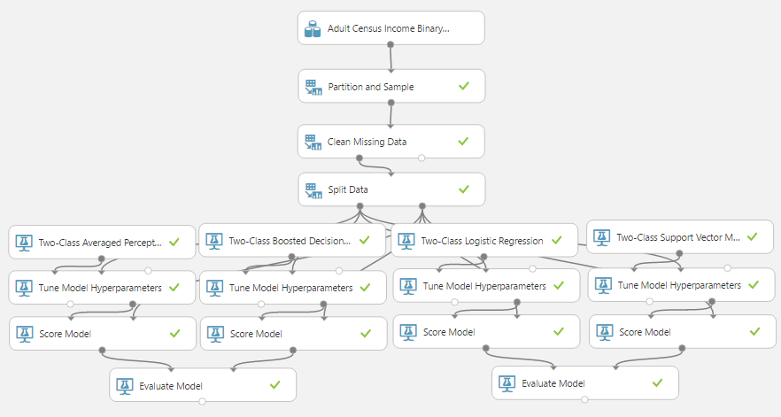
| Experiment |
As a quick refresher, we are training and scoring four models using a 70/30 Training/Testing split, stratified on "Income". Then, we are evaluating these models in pairs. For a more comprehensive description, feel free to read the
ROC post. Let's move on to the "Evaluate Model" visualization.
 |
| Threshold and Evaluation Tables |
At the bottom of all of the tabs, there are two tables. We've taken to calling them the "Threshold" and "Evaluation" tables. If these tables have legitimate names, please let us know in the comments. Let's start by digging into the "Threshold" table.
 |
| Threshold Table |
On this table, we can use the slider to change the "Threshold" value to see what effect it will have on our summary statistics. Some of you might be asking "What is this threshold?" To answer that, let's take a look at the output of the "Score Model" module that feeds into the "Evaluate Model" module.
 |
| Scores |
At the end of every row in the output, we find two columns, "Scored Labels" and "Scored Probabilities". The "Scored Probabilities" are what the algorithm has decided is the probability that this record belongs to the TRUE category. In our case, this would be the probability that the person has an Income of greater than $50k. By default, "Scored Labels" predicts TRUE if the probability is greater .5 and FALSE if it isn't. This is where the "Threshold" comes into play. We can use the slider from the Threshold table to see what would happen if we were to utilize a stricter threshold of .6 or a more lenient threshold of .4. Let's look back at the Threshold table again.
 |
| Threshold Table |
Looking at this table, we can see the total number of predictions in each category, as well as a list of Accuracy metrics (
Accuracy,
Precision, Recall and
F1). Threshold selection can be a very complicated process based on the situation. Let's assume that we're retailers trying to target potential customers for an advertisement in the mail. In this case, a False Positive would mean that we sent an advertisement to someone who will not buy from us. This wastes a few pennies because mailing the advertisement is cheap. On the other hand, a False Negative would mean that we didn't send an advertisement to someone who would have bought from us. This misses the opportunity for a sale, which is worth much more than a few pennies. Therefore, we are more interested in minimizing False Negatives than False Positives. This causes situations where using the built-in metrics may not be the best decision. In our case, let's just assume that overall "Accuracy" is what we're looking for. Therefore, we want to maximize as many of these metrics as we can.
Also, there's another metric over to the side called "AUC". This stands for "
Area Under the Curve". For those of you that read our
ROC post, you may remember that our goal was to find the chart that was closer to the top left. Mathematically, this is equivalent to finding the curve that represents the largest area. Let's take a look at a couple of different thresholds.
 |
| Threshold Table (T = .41) |
 |
| Threshold Table (T = .61) |
The first thing we notice is that the "Positive Label", "Negative Label", and "AUC" do not change. "Positive Label" and "Negative Label" are displayed for clarity purposes and "AUC" is used to compare different models to each other. None of these are affected by the threshold. Remember that earlier we decided that "Accuracy" was our metric of interest. Using the default threshold of .5, as well as the altered thresholds of .41 and .61, we can see that there is less than 1% difference between these values. Therefore, we can say that there is virtually no difference in "Accuracy" between these three thresholds. If this was a real-world experiment, we could reexamine our problem to determine whether another type of metric, such as "Precision", "Recall", "F1 Score" or even a custom metric would be more meaningful. Alas, that discussion is better suited for its own post. Let's move on.
As you can imagine, this table is good for looking at individual thresholds, but it can get time-consuming quickly if you are trying to find the optimal threshold. Fortunately, there's another way, let's take a look at the "Evaluation" Table.
 |
| Evaluation Table |
This table is a bit awkard and took us quite some time to break down. In reality, it's two different tables. We've recreated them in Excel to showcase what's actually happening.
 |
| Discretized Results |
The "Score Bin", "Positive Examples" and "Negative Examples" columns make up a table that we call the "Discretized Results". This shows a breakdown of the Actual Income Values for each bucket of Scored Probabilities. In other words, this chart says that for records with a Scored Probability between .900 (90%) and 1.000 (100%), 50 of them had an Income value of ">50k" and 4 had an Income value of "<=50k".
 |
| Discretized Results (Augmented) |
Since the algorithm is designed to identify Incomes of ">50k" with high probabilities and Incomes of "<=50k" with low probabilities, we would expect to see most of the Positive Examples at the top of the table and most of the Negative Examples at the bottom of the table. This turns out to be true, indicating that our algorithm is "good". Now, let's move on to the other part of the Evaluation Table.
 |
| Evaluation Table |
 |
| Threshold Results |
We can use the remaining columns to create a table that we're calling the "Threshold Results". This table is confusing for one major reason. None of the values in this table are based on the ranges defined in the "Scored Bin" column. In reality, these values are calculated by utilizing a threshold
equal to the value at the bottom of the threshold defined in the "Score Bin" column. To clarify this, we've added a column called "Threshold" to showcase what's actually being calculated. To verify, let's compare the Threshold table to the Threshold Results for a threshold of 0.
 |
| Threshold Table (T = 0) |
We can see that the "Accuracy", "Precision", "Recall" and "F1 Score" match for a threshold of 0 using the last line of the Evaluation Table. Initially, this was extremely confusing to us. However, now that we know what's going on, it's not a big deal. Perhaps they can alter this visualization in a future release to be more intuitive. Let's move back to the Threshold Results.
 |
| Threshold Results |
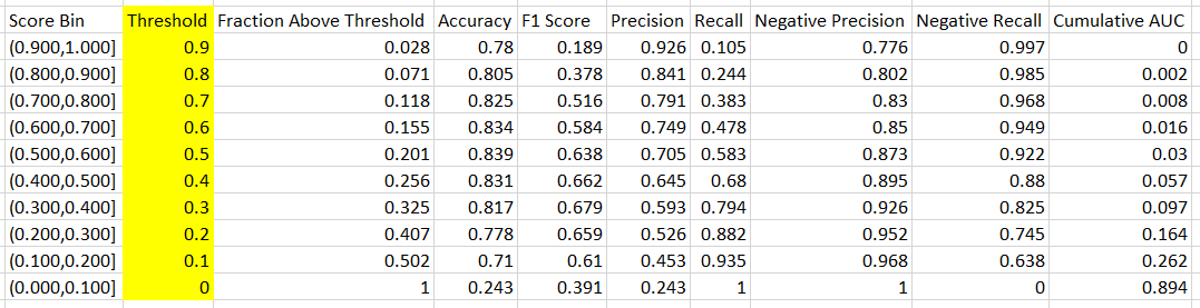
Let's talk about what these columns represent. We've already talked about the "Accuracy", "Precision", "Recall" and "F1 Score" columns. The "Negative Precision" and "Negative Recall" are similar to "Precision" and "Recall", except that they are looking for Negative values (Income = "<=50k") instead of Positive values (Income = ">50k"). Therefore, we're looking maximize all six of these values.
The "Fraction Above Threshold" column tells us what percentage of our records have Scored Probabilities greater than the Threshold value. Obviously, all of the records have a Scored Probability greater than 0. However, it is interesting to note that 50% of our values have Scored Probabilities between 0 and .1. This isn't surprising because, as we mentioned in a previous
post, the Income column is an "Imbalanced Class". This means that the values within the column are not evenly distributed.
The "Cumulative AUC" column is a bit more complicated. Earlier, we talked about "AUC" being the area under the ROC curve. Let's take a look at how a ROC curve is actually calculated.
 |
| ROC Curve |
The ROC Curve is calculated by selecting many different threshold values, calculating the True Positive Rate and False Positive Rate, then plotting all of the points as a curve. In the above illustration, we show how you might use different threshold values to define points on the red curve. It's important to note that our threshold lines above were not calculated, they were simply drawn to illustrate the methodology. Looking at this, it's much easier to understand "Cumulative AUC".
Simply put, "Cumulative AUC" is the area under the curve up to a particular threshold value.
 |
| Cumulative AUC (T = .5) |
This opens up another interesting option. In the previous posts (
ROC and
Precision/Recall and Lift), we evaluated multiple models by comparing them in pairs and comparing the winners. Using the Evaluation Tables, we could compare all of these values simultaneously in Excel. For instance, we could use Cumulative AUC to compare all four models at one.
 |
| Cumulative AUC Comparison |
Using this visualization, we can see that the Boosted Decision Tree is the best algorithm for anything thresholds greater than .3 (30%) or less than .1 (10%). If we wanted to utilize a threshold within these values, we would be better off using the Averaged Perceptron or Logistic Regression algorithms. Hopefully, we've sparked your imagination to explore all the capabilities that Azure ML has to offer. It truly is a great tool that's opening the world of Data Science beyond just the hands of Data Scientists. Thanks for reading. We hope you found this informative.
Brad Llewellyn
Data Scientist
Valorem
@BreakingBI
www.linkedin.com/in/bradllewellyn
llewellyn.wb@gmail.com