Today, we're going to expand on our previous
post. In the previous post, we built a simple data model using a sample data set. However, there were a few situations that we cheated through for simplicity's sake. Today, we're going to reformat the Users table using Power Query.
 |
| Users (Original) |
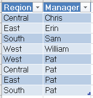
The original users table had 4 rows for the 4 different managers with their corresponding regions. It also had 4 additional rows for the CEO, Pat. This formatting would cause huge problems if you were to join or link to this table. In fact, Power BI prohibits us from doing this.
 |
| Cannot Create Relationship |
If we were to somehow force Power BI to create this relationship, which we're not even sure we can do, it would cause headaches when we tried to use these fields in our charts and calculations. We could create a pivot table that would correctly show the sales for each of the 4 managers. It would also correctly show the sales for Pat as the sum of the sales for all the managers. However, our total sales should be the sales for Pat; but, Power BI would actually show us twice that as our total sales because it would be summing the 4 managers' sales with Pat's sales to get the total sales. This is called a "Many-to-Many" relationship and needs to handled in a very different way. Alas, that's not the purpose of this post. We want to reformat this table so that it has 4 unique rows (1 for each region), with a column for the Manager of that region, and a column for CEO (which is Pat). In order to do this, we need to use Power Query to edit the data as it's coming in.
 |
| Edit Queries |
We begin by clicking the "Edit Queries" button in the Ribbon. This opens up the Power Query window.
 |
| Users (Bad Headers) |
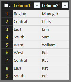
The first thing we notice is that the headers did not come through properly. We can easily fix that by clicking the "Use First Row as Headers" button in the Ribbon.
 |
| Use First Row As Headers |
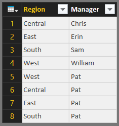
This fixes the headers, but we still have the issue with Pat's rows.
 |
| Users (Good Headers) |
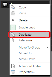
Let's start by duplicating this query by right-clicking on Users in the left Query panel, and selecting the "Duplicate" option. This will create a Users (2) table that is identical to the Users table, for now.
Next, let's summarize the Users (2) table to show the Number of Regions per Manager. We can accomplish by clicking the "Group By" button the Ribbon.
 |
| Group By |
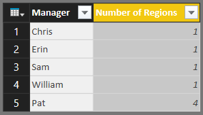
Next, we choose to create the "Number of Regions" column via grouping by "Manager" and using the "Count Rows" calculation.
 |
| Number of Regions |
Now, our Users table shows the Number of Regions for each Manager.
 |
| Users (Number of Regions) |
Now, we need to be able to identify who the CEO is and who the regular managers are. This table is great for that because we know that anyone with a "Number of Regions" equal to 1 is a manager, while the user with "Number of Regions" equal to 4 is a CEO. Next, we need to join/merge these two tables together. We can do that by clicking the "Merge Queries" button in the Ribbon.
 |
| Merge Queries |
Now, we need to select the table we would like to join to, as well as the column we would like to join on, and the type of join we would like to perform. Since we only have 2 tables, we want to join Users to Users (2). We also have to join on Manager because that is the only column they have in common. Finally, we have quite a few options for which join we perform. Since we created the Users (2) table from the Users table with no filters, we know that every manager in Users is also in Users (2), and vice-versa, that means that Inner Join, Left Outer Join, Right Outer Join, and Full Outer Join will give us the same result. For simplicity, let's just choose Inner Join.
 |
| Merge |
Now, we have the information from Users (2) in the Users table.
 |
| Users (Merged, Dirty) |
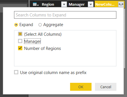
Currently, we can't see the information that was merged into this table. So, we need to expand the "Table" by clicking on the "Double Arrow" at the top of the NewColumn and selecting the "Number of Regions" checkbox in the "Expand" panel. Also, it's cleaner if you deselect the "Use Original Column Name as Prefix" option.
 |
| Expand Number of Regions |
This leaves us with a table that looks more traditional.
 |
| Users (Merged, Clean) |
Now, we have a way to identify who is a CEO and who is a Manager. So, let's create a calculated column that shows that. We can do this by selecting the "Add Custom Column" button in the "Add Column" Ribbon.
 |
| Add Custom Column |
Next, we need to define our calculation. The language behind Power Query is formerly known as "M". You can find a formula library
here. We want to create a calculation called "Level" that returns "CEO" if "Number of Regions" equals 4, and returns "Manager" otherwise.
 |
| Level |
This calculation adds the "Level" column to the Users table.
 |
| Users (with Level) |
Here's where we get to the tricky part. We want to transform this table so that it contains a column for Manager and a column for CEO. The manager column should have the appropriate manager based on the region, while the CEO column always has Pat. We can accomplish this by selecting the "Level" column, then clicking the "Pivot Column" button in the "Transform" Ribbon.
 |
| Pivot Column |
Now, we've already told Power Query that we want to create columns based on the values in the "Level" column. However, we still need to tell it what values should go in the new columns. We want the new columns to take the non-aggregated values from the Manager column, i.e. the Manager Names.
 |
| Pivot Level with Manager |
Now, our table has quite a few holes.
 |
| Users (with Holes) |
Most programming languages, including SQL, will aggregate values when you perform a pivot to remove holes like this. Unfortunately, Power Query does not. There are a number of ways we could accomplish this. We think the easiest way is to select the "CEO" column, then select the "Fill Up" button in the "Transform" Ribbon.
 |
| Fill Up |
This will fill in the gaps in the CEO column. We could use "Fill Down" to fill the gaps in the Manager column as well. However, we don't need to. We're only interested in having a single row for each Region, with the corresponding Manager and CEO listed. Looking down the list, we see that we already have these 4 rows available.
 |
| Users (Filled) |
So, all we have to do is filter the "Number of Regions" column to only include 1. We can do that by clicking the Triangle at the top of the column, and deselecting the "4" box.
 |
| Filter Number of Regions |
Now, our table looks almost ready.
 |
| Users (Filtered) |
All that's left to do is the remove the "Number of Regions" column because we no longer need it. We can do that by selecting the "Number of Regions" column and clicking the "Remove Columns" button from the "Home" Ribbon.
 |
| Remove Columns |
Now, our table is complete and we can use it to further our analysis.
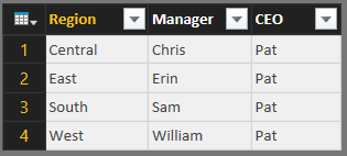 |
| Users (Clean) |
The interesting thing about this procedure is that it can likely be done in a myriad of other ways. Power Query even has an advanced editor where you could probably code an approach to handle this automatically. We definitely didn't take the easy way out for accomplishing this. To see that, check out our previous
post. All in all, we feel this approach is pretty flexible, but lacks some of the more advanced features. For instance, what if there were 3 levels of hierarchy in our instead of just the 2 we had here (Manager and CEO)? Could we create some sort of iterative process to accomplish this? Maybe someone in the comments can help us out. Thanks for reading. We hope you found this informative.
Brad Llewellyn
BI Engineer
Valorem Consulting
@BreakingBI
www.linkedin.com/in/bradllewellyn
llewellyn.wb@gmail.com