Today, we're going to talk about how to set up a simple data model in Power BI Desktop and PowerPivot. The data set we are going to be using can be found
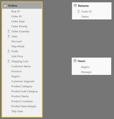
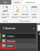
here. Simply put, a data model is a set of tables designed to work together. For instance, having a table showing all of your sales is great. However, what if you want to compare your sales across different product lines, but your product line information is in a different table? This is the type of situation we're going to solve today by building a simple data model. Every data model starts by looking at your data. Our dataset consists of 3 tables, Orders, Returns, and Users.
 |
| Orders |
 |
| Returns |
 |
| Users |
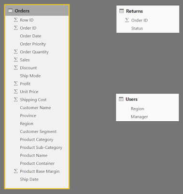
The Orders table contains transaction data about each order. This includes the products that were purchased, how much they paid for them, when they purchased them, etc. This is an extremely common type of table that exists in virtually every business. Next, the Returns table is a lookup table letting us know which orders were returned. Lastly, the Users table shows us which managers are assigned to which regions. Let's start by pulling all of the tables into Power BI Desktop.
 |
| Data Model (No Connections) |
Power BI tries to find relationships between the tables and make connections. Fortunately for us, it didn't find any. This means that we get to walk through the process from the beginning. Generally, the purpose of a data model is to connect lookup tables to transaction tables. Depending on the style of data architecture being used, these tables may also be referred to as Facts and Dimensions. Simply put, your Transaction or Fact tables contain the values you want to aggregate (sum, count, average, etc.) and your Lookup or Dimension tables contain the values you want to slice, filter, or group by. For more information on Facts and Dimensions, check out
this link or google Kimball vs. Inmon.
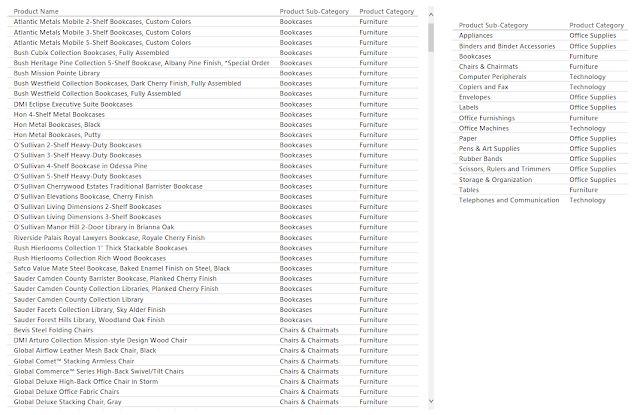
Now that we've identified what each of the tables are, we can start looking at how "clean" they are. "Clean" is a term that generally refers to how usable a data set is for a specific purpose. For data modeling, you generally want your transaction tables to be flat. This means that each column should be a unique metric or slicer. Imagine that we had a dataset that contained a column for "2011 Sales" and "2012 Sales". We would want to pivot those down to a year column taking the values 2011 and 2012, and a Sales column that takes the appropriate value from the old columns. In our case, the data set is clean enough for an introduction. One thing that does stick out is the Product Hierarchy. There are columns for Product Category, Product Sub-Category, and Product Name.
 |
| Product Hierarchy |
If we look through the hierarchy, we can see that each Product Name exists in only 1 Product Sub-Category and each Product Sub-Category exists in only 1 Product Category. This means that they form a perfect hierarchy. Best practices suggest that these values should be split into their own lookup table(s). However, this is a more advanced process that we'll handle in a later post. There is a task that we need to take care of now though. If we look at the Orders table in the Relationships canvas, we see that quite a few columns are flagged with a Sigma (
∑).
 |
| Data Model (No Connections) |
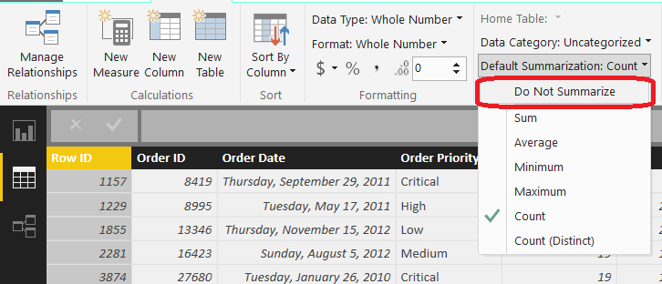
When the data set was imported, Power BI looked at these columns and decided that they should be aggregated because they are numeric. For columns like Sales, this is true. However, we have some columns that are actually numeric slicers, such as Discount and Product Base Margin, as well as numeric keys, such as Row ID and Order ID. These columns should not be aggregated. We can fix this by moving on to the Data canvas and changing the Default Summarization for each of these columns.
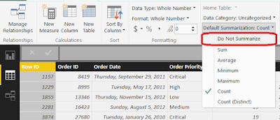 |
| Do Not Summarize |
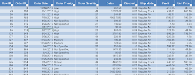
Doing this for all appropriate columns leave us with a very different picture of the table in the Relationships canvas.
 |
| Data Model (Clean Orders) |
Now, we can call the Orders table clean enough for our needs and move on to the Returns table.
 |
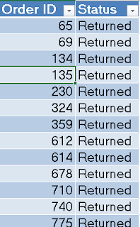
| Returns |
This table shows each Order ID that was Returned. In many transactional systems, another row would be added to the transaction table with a negative value and quantity to show that an item was returned. Doing so would allow all metrics to still calculate correctly, while still having the evidence of a return. This is another case that we'll have to cover in another post. In our case, we'll leave it like it is. Finally, we recognize that Order ID is a key column. Key columns are used to connect tables to each other. In a perfect model, you would like a key to be unique in the lookup table but not unique in the transaction table. This is not always the case in the real world, but it happens to be here. Each Order ID appears only once in the Returns table. Just like before, we need to change the Default Summarization of Order ID so that Power BI does not attempt to aggregate it.
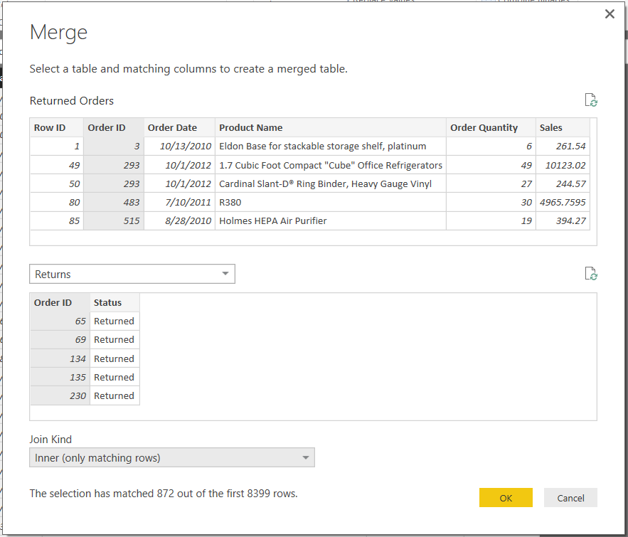
Next, we need to connect the Returns table to the Orders table. In Power BI Desktop, this is a simple task.
 |
| Data Model (Clean Returns) |
First, open the Relationships canvas.
 |
| Create Connection |
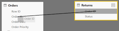
Next, click-drag "Order ID" from the Returns table onto "Order ID" from the Orders table.
 |
| Data Model (Connected Returns) |
This created a "one-to-many" relationship from Returns to Orders. This is exactly what we wanted. Now, we can create charts using "Status" as a slicer against measures from the Orders table. Let's move on to the Users table.
 |
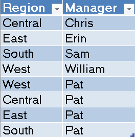
| Users |
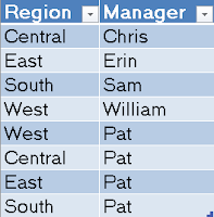
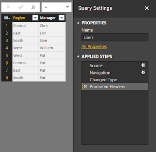
This table is a bit more interesting. We have each of the managers tied to their respective regions. However, we also have the CEO Pat tied to every region. This means that Region is not a unique key in this table. We want to remove Pat's rows from the bottom of the table, and add a new column labeled CEO which would take the value "Pat" for all 4 rows. There are some great ways to handle this using the Query editor (also known as Power Query). However, we'll take the easy way this time and save the hard work for a later post.
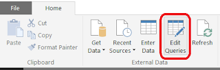
Let's start by opening the Query Editor.
 |
| Edit Queries |
The query editor is where you can edit your Data Import queries in a number of ways to get exactly the format you want. Let's open the Query for the Users table.
 |
| Select Users Query |
This shows us what the Users table currently looks like, as well as shows us every step that was taken to create it.
 |
| Users Query |
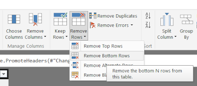
Since we didn't mess with the queries, all of the steps listed are the defaults. What we want to do is remove the bottom 4 rows. We can do this by selecting the "Remove Bottom Rows" option from the toolbar and typing in the number 4.
 |
| Remove Bottom Rows |
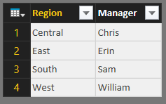
This leaves us with only the legitimate managers in the table.
 |
| Users Table (Legit) |
Now, we apply these changes and go back to our model.
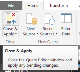 |
| Close and Apply |
Next, we need to add the CEO column and give it the value "Pat" for all rows. We start by navigating to the Data canvas and select the "New Column" button.
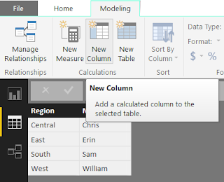 |
| New Column |
Next, we type the function CEO = "Pat" into the function bar.
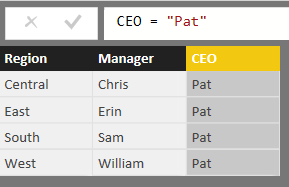 |
| Users Table (Clean) |
This will automatically rename the column to CEO and populate it with "Pat" for every row. Finally, we need to connect this table to the Orders table using the Region key.
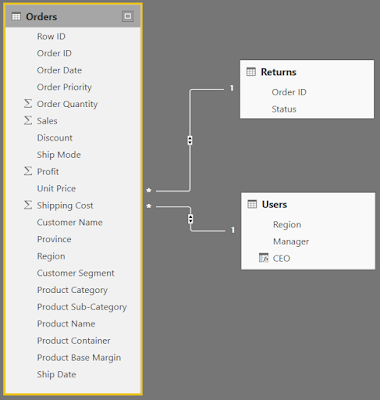 |
| Data Model (Complete) |
Now, we can slice and dice our Orders data by any of the slicers we want, including the slicers in the Returns and Users tables. Hopefully, this opened your eyes to how easy it is to build simple data models in Power BI Desktop. Stay tuned for later posts where we get more in-depth on how to handle these problems using best practices, as well as deal with more difficult issues. Thanks for reading. We hope you found this informative.
Brad Llewellyn
BI Engineer
Valorem Consulting
@BreakingBI
www.linkedin.com/in/bradllewellyn
llewellyn.wb@gmail.com