Today, we're going to continue with our Fraud Detection experiment. If you haven't read our previous posts in this series, it's recommended that you do so. They cover the
Preparation,
Data Cleansing and
Model Selection phases of the experiment. In this post, we're going to walk through the model evaluation process.
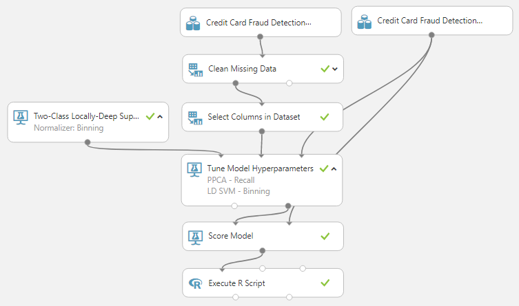
Model evaluation is "where the rubber meets the road", as they say. Up until now, we've been building a large list of candidate models. This is where we finally choose the one that we will use. Let's take a look at our experiment so far.
 |
| Experiment So Far |
We can see that we have selected two candidate imputation techniques and fourteen candidate models. However, the numbers are about get much larger. Let's take a look at the workhorse of our experiment, "Tune Model Hyperparameters".
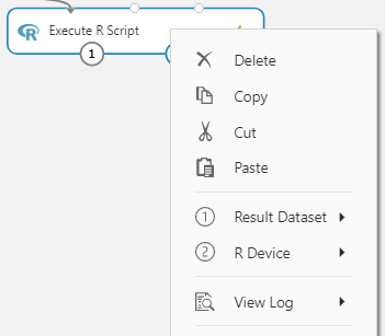
 |
| Tune Model Hyperparameters |
We've looked at this module in some of our previous posts (
here and
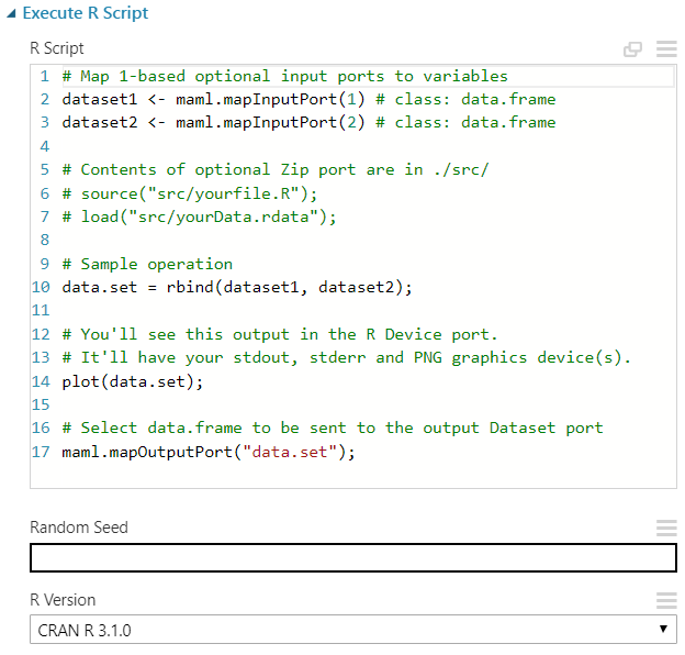
here). Basically, this module works by allowing us to define (or randomly choose) sets of hyperparameters for our models. For instance, if we run the "Two-Class Boosted Decision Tree" model through this module with our training and testing data, we get an output that looks like this.
 |
| Sweep Results (Two-Class Boosted Decision Tree) |
The result of the "Tune Model Hyperparameters" module is a list of hyperparameter sets for the input model. In this case, it is a list of hyperparameters for the "Two-Class Boosted Decision Tree" model, along with various evaluation metrics. Using this module, we can easily test tens, hundreds or even thousands of different sets of hyperparameters in order to find the absolute best set of hyperparameters for our data.
Now, we have a way to choose the best possible model. The next step is to choose which evaluation metric we will use to rank all of these candidate models. The "Tune Model Hyperparameters" module has a few options.
 |
| Evaluation Metrics |
This is where a little bit of mathematical background can help tremendously. Without going into too much detail, there's a problem with using some of these metrics on our dataset. Let's look back at our "Class" variable.
 |
| Class Statistics |
 |
| Class Histogram |
We see that the "Class" variable is extremely skewed, with 99.87% of all observations having a value of 0. Therefore, traditional metrics such as Accuracy and AUC are not acceptable. To further understand this, imagine if we built a model that always predicted 0. That model would have an accuracy of 99.87%, despite being completely useless for our use case. If you want to learn more, you can check out this
whitepaper. Now, we need to utilize a new set of metrics. Let's talk about
Precision and Recall.
Precision is the percentage of predicted "positive" records (Class = 1 -> "Fraud" in our case) that are correct. Notice that we said
PREDICTED. Precision looks at the set of records where the model thinks Fraud has occurred. This metric is calculated as
(Number of Correct Positive Predictions) / (Number of Positive Predictions)
One of the huge advantages of Precision is that it doesn't care how "rare" the positive case is. This is extremely beneficial in our case because, in our opinion, 0.13% is extremely rare. We can see that we want precision to be as close to 1 (or 100%) as possible.
On the other hand,
Recall is the percentage of actual "positive" records that are correct. This is slightly different from Precision in that it looks at the set of records where Fraud has actually occurred. This metric is calculated as
(Number of Correct Positive Predictions) / (Number of Actual Positive Records)
Just as with Precision, Recall doesn't care how rare the positive case is. Also like Precision, we want this value to be as close to 1 as possible.
In our minds, Precision is a measure of how accurate your fraud predictions are, while Recall is a measure of how much fraud the model is catching. Let's look back at our evaluation metrics for the "Tune Model Hyperparameters" module.
 |
| Evaluation Metrics |
We can see that Precision and Recall are both in this list. So, which one do we choose? Honestly, we don't have an answer for this. So, we'll go back to our favorite method, try them both!
 |
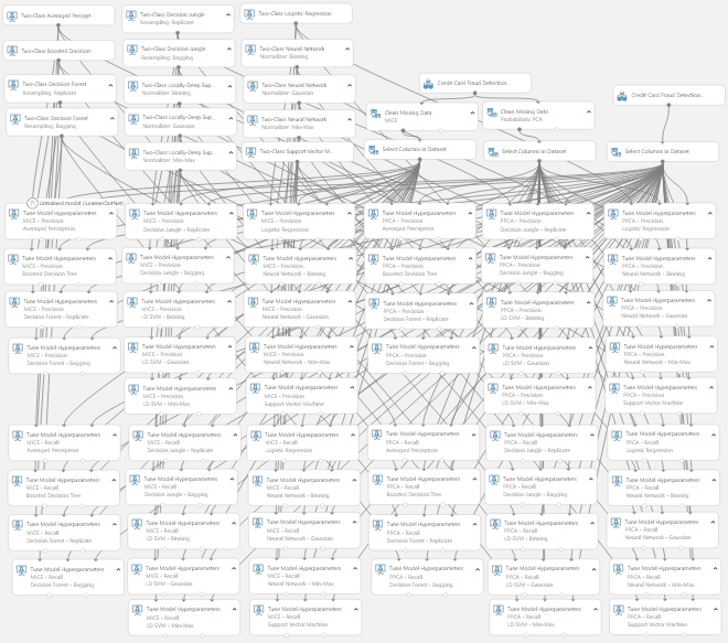
| Model Evaluation Experiment |
This is where Azure Machine Learning really provides value. In about thirty minutes, we were able to set up this experiment that's going to create two evaluation metrics against fourteen sets of twenty models utilizing two cleansing techniques. That's a total of 1,120 models! After this finishes, we copy all of these results out to an Excel spreadsheet so we can take a look at them.
 |
| MICE - Precision - Averaged Perceptron Results |
Our Excel document is simply a series of tables very similar to this one. They show the parameters used for the model, as well as the evaluation statistics for that model. Using this, we could easily find the combination of model, parameters and cleansing technique that gives us the highest Precision or Recall. However, this still requires us to choose one or the other. Looking back at the definitions of these metrics, they cover two different, important cases. What if we want to maximize both? Since we have the data in Excel, we can easily add a column for Precision * Recall and find the model that maximizes that value.
 |
| PPCA - Recall - LD SVM - Binning Results |
As we can see from this table, the best model for this dataset is to clean the data using Probabilistic Principal Component Analysis, then model the data using a Locally-Deep Support Vector Machine with a Depth of 4, Lambda W of .065906, Lambda Theta Prime of .003308, Sigma of .106313 and 14,389 Iterations. A very important consideration here is that we will not get the same results by copy-pasting these parameter values into the "Locally-Deep Support Vector Machine" module. That's because these values are rounded. Instead, we should save the best module directly to our Azure ML workspace.
 |
| Save Trained Model |
At this point, we could easily consider this problem solved. We have created a model that catches 90.2% of all fraud with a precision of 93.0%. A very important point to note about this whole exercise is that we did not use domain knowledge, assumptions or "Rules of Thumb" to drive our model selection process. Our model was selected entirely by using the data. However, there are a few more steps we can perform to tweak more power and performance out of our model. Hopefully, this has opened your eyes to the Model Evaluation power of Azure Machine Learning. Stay tuned for the next post where we'll discuss Threshold Selection. Thanks for reading. We hope you found this informative.
Brad Llewellyn
Data Scientist
Valorem
@BreakingBI
www.linkedin.com/in/bradllewellyn
llewellyn.wb@gmail.com