Data Cleansing is arguably one of the most important phases in the Machine Learning process. There's an old programming adage "Garbage In, Garbage Out". This applies to Machine Learning even more so. The purpose of data cleansing is to ensure that the data we are using is "suitable" for the analysis we are doing. "Suitable" is an amorphous term that takes on drastically different meanings based on the situation. In our case, we are trying to accurately identify when a particular credit card purchase is fraudulent. So, let's start by looking at our data again.
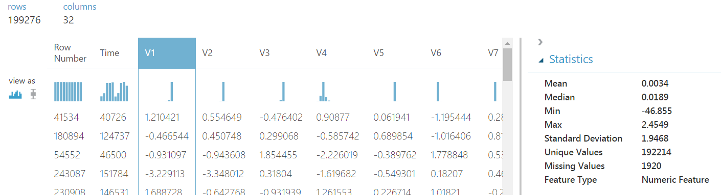 |
| Credit Card Fraud Data 1 |
 |
| Credit Card Fraud Data 2 |
 |
| Class Statistics |
 |
| Class Histogram |
 |
| Credit Card Fraud Summary 1 |
 |
| Credit Card Fraud Summary 2 |
 |
| Credit Card Fraud Summary 3 |
 |
| Clean Missing Data |
In the previous posts, we've focused on "Custom Substitution Value" just to save time. However, our goal in this experiment is to create the most accurate model possible. Given that goal, it would seem like a waste not to use some of more powerful tools in our toolbox. We could use some of the simpler algorithms like Mean, Median or Mode. However, we have a large number of dense features (this is a result of the Principal Component Analysis we talked about in the previous post). This means that we have a perfect use case for the heavy-hitters in the toolbox, MICE and Probabilistic PCA (PPCA). Whereas the Mean, Median and Mode algorithms determine a replacement value by utilizing a single column, the MICE and PPCA algorithm utilize the entire dataset. This makes them extremely powerful at providing very accurate replacements for missing values.
So, which should we choose? This is one of the many crossroads we will run across in this experiment; and the answer is always the same. Let the data decide! There's nothing stopping us from creating two streams in our experiment, one which uses MICE and one which uses PPCA. If we were so inclined, we could create additional streams for the other substitution algorithms or a stream for no substitution at all. Alas, that would greatly increase the development effort, without likely paying off in the end. For now, we'll stick with MICE and PPCA. Which one's better? We won't know that until later in the experiment.
Hopefully, this post enlightened you to some of the ways that you can use Imputation and Data Cleansing to provide additional power to your models. There was far more we could do here. In fact, many data scientists approaching hard problems will spend most of their time adding new variables and transforming existing ones to create even more powerful models. In our case, we don't like putting in the extra work until we know it's necessary. Stay tuned for the next post where we'll talk about model selection. Thanks for reading. We hope you found this informative.
Brad Llewellyn
Data Scientist
Valorem
@BreakingBI
www.linkedin.com/in/bradllewellyn
llewellyn.wb@gmail.com