Today, we're going to walk through the In/Out Tools.
Input Tool 1: Input Data
 |
| Input Data |
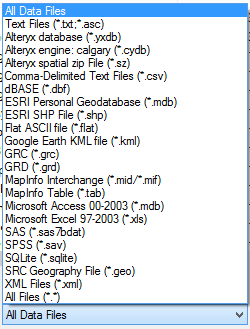 |
| Input File Types |
Basically, this covers most of the files you are going to find. If you need to connect to a database, they allow you to create your own connections, similarly to the way Excel does it.
 |
| Database Connection |
Input Tool 2: Map Input
 |
| Map Input |
This is probably the coolest input tool, albeit the least useful for real analysis. It allows you to select point, draw lines, or create polygons by drawing with your mouse. You can even use a map as the base to draw polygons around geographic areas. For instance, if you wanted to point out key locations on a map, or draw a polygon around a location or set of locations.
 |
| Statue of Liberty |
You can even import your own Alteryx Database (YXDB) files to use as a start.
 |
| Ad Areas |
This tool is really useful for cool presentations. But, we don't see it having much analytical use other than estimating locations of things for geocoding purposes.
Input Tool 3: Text Input
 |
| Text Input |
This tool is really useful when you need to relabel or append data on a one-off basis. Let's say that you have a file with all of your customers and you need to Categorize them according to a complex list. You could create that list with a Text Input and join it to your original data.
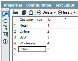 |
| Customer Types |
If you have the ability to change the original data, you should definitely add this there. You could also create a separate Excel file with just this table so that you can use it in other places as well. If for some reason you can't do any of that, then the Text Input tool is a quick alternative.
We actually had a case where we created a complex R macro that always required at least 1 row of data. However, some times we would not have any data to give it. So, we added a Text Input with a blank row and appended it to the data source. This way, there was always at least 1 row in the data set. Alas, this is a very situational tool.
Input Tool 4: Directory
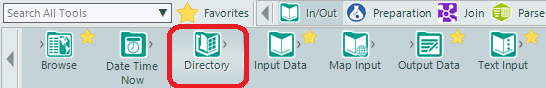 |
| Directory |
This tool allows you to input the file names, paths, and a myriad of other data about the files within a certain folder on your hard drive or server.
 |
| Directory Properties |
This is useful for determining the last time certain files are updated and how often people are writing files to a directory. Combined with the Dynamic Input tool, you can use this to import multiple files within multiple directories using very complex logic. This could allow to keep track of all your data in a single place without having to archive it in a single folder. There's a Sample Module in Alteryx that uses this tool to a similar purpose.
Input Tool 5: Date Time Now
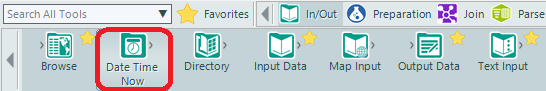 |
| Date Time Now |
This tool hardly needs an explanation. You tell it the format, and it outputs the Date and Time that your Alteryx Module runs.
 |
| Date Time Now Properties |
This is great if you want to track the times that a module or finding which pieces of a macro or module are taking a long time. Interestingly enough, the Formula tool can give you this same information in a more efficient way. Therefore, we can't think of too many cases where this tool would be useful.
Output Tool 1: Browse
 |
| Browse |
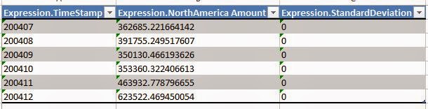
This is the most common tool you will use in Alteryx. It allows to you to view the data being passed through any section of your Alteryx module. It can even view charts, visualizations, and maps.
 |
| Pet Store Monthly Sales |
If you want to save this data for later, you can copy it to the clipboard or save it to one of the output file types.
 |
| Save Browse |
Output Tool 2: Output Data
 |
| Output Data |
This tool is great if you want to output files without the manual work of using the Browse tool. It can output a pretty comprehensive list of file types.
 |
| Output File Types |
You can even name the file using a field within the data if you want to use this tool within some type of Iterative or Batch Macro. The big thing to note here is that Alteryx can output proprietary file types like Tableau Data Extracts, QlikView data eXchanges, and ESRI SHP Files.
As you can see, Alteryx is pretty sophisticated when it comes to reading in and writing out different types of data. The real power of the tool comes when you quickly join the data together and create advanced analyses. Stay tuned for the next post where we'll be talking about the Field Preparation tools. Thanks for reading. We hope you found this informative.
Brad Llewellyn
Director, Consumer Sciences
Consumer Orbit
llewellyn.wb@gmail.com
Director, Consumer Sciences
Consumer Orbit
llewellyn.wb@gmail.com
http://www.linkedin.com/in/bradllewellyn
.JPG)
.JPG)


.JPG)
.JPG)
.JPG)
.JPG)


.JPG)

.JPG)


.JPG)


.JPG)
