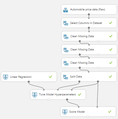
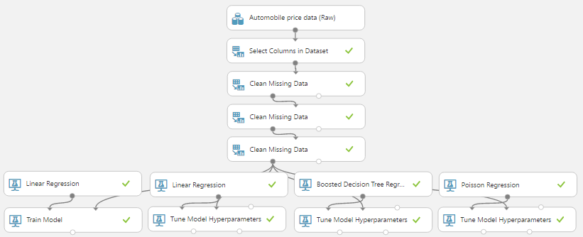
Monday, May 15, 2017

Azure Machine Learning: Regression Model Evaluation

Today, we're going to continue our walkthrough of Sample 4: Cross Validation for Regression: Auto Imports Dataset.  In the previous posts, we walked through the Initial Data Load, Imputation, Ordinary Least Squares Linear Regression, Online Gradient Descent Linear Regression, Boosted Decision Tree Regression and Poisson Regression phases of the experiment.
Experiment So Far
Let's refresh our memory on the data set.
Automobile Price Data (Clean) 1

Automobile Price Data (Clean) 2
We can see that this data set contains a bunch of text and numeric data about each vehicle, as well as its price.  The goal of this experiment is to attempt to predict the price of the car based on these factors.  While there are more regression techniques available in Azure ML, we're going to talk about the steps for evaluating our regression models.  Let's start by talking about Testing and Training Sets.

So far in our experiment, we've trained our models using the entire data set.  This is great because it gives the algorithm as much information as possible to make the best possible model.  Now, let's think about how we would test the model.  Testing the model, also known as model evaluation, requires that we determine how well the model would predict for data it hasn't seen yet.  In practice, we could easily train the model using the entire dataset, then use that same dataset to test the model.  However, that would determine how well the model can predict for data is has already seen, which is not the purpose of testing.

The most common approach to alleviate this issue is to split your data into two different sets, a Training Set and a Testing Set.  The Training Set is used to train the model and the Testing Set is used to test the model.  Using this methodology, we are testing the model with data it hasn't seen yet, which is the entire point.  To do this, we'll use the "Split Data" module.
Split Data
For this experiment, we'll be using "Split Rows" as our "Splitting Mode".  The other choices are more complex.  You can read about them here.

The "Fraction of Rows in the First Output Dataset" defines how many rows will be passed through the left output of the module.  In our case, we'll use .7 (or 70%) of our data for our Training Set and the remaining 30% for our Testing Set.  This is known as a 70/30 split and is generally considered the standard way to split.

The "Randomized Split" option is very important.  If we were to deselect this option, the first segment of our rows (70% in this case) would go through the left output and the last segment (30% in this case) would go through the right side.  Ordinarily, this is not what we would want.  However, there may be some obscure cases where you could apply a special type of sorting beforehand, then use this technique to split the data.  If you know of any other reasons, feel free to leave us a comment.

The "Random Seed" option allows us to split our data the same way every time.  This is really helpful for demonstration and presentation purposes.  Obviously, this parameter only matters if we have "Randomized Split" selected.

Finally, the "Stratified Split" option is actually quite significant.  If we select "False" for this parameter, we will be performing a Simple Random Sample.  This means that Azure ML will randomly choose a certain number of rows (70% in our case) with no regard for what values they have or what order they appeared in the original dataset.  Using this method, it's possible (and actually quite common) for the resulting dataset to be biased in some way.  Since the algorithm doesn't look at the data, it has no idea whether it's sampling too heavily from a particular category or not.
Price (Histogram)
If we look at the "Price" column in our dataset, we see that it is heavily right-skewed.  If we were to perform a Simple Random Sample on this data, it very possible that we could miss most (if not all) of the vehicles with high prices.  This would bias our sample toward vehicles with lower prices, potentially hurting our predictive ability.
Split Data (Stratified)
One way to alleviate this is to perform a Stratified Sample.  This can be accomplished by selecting "True" for the "Stratified Split" option.  Next, we need to select a column (or set of columns).  Basically, Azure ML will break the data up into segments based on the unique values in the select column (or combination of columns).  Then, it will perform a Simple Random Sample on each segment.  This can be extremely helpful if your data set has some extremely important factors that need to have the similar distributions in the Training Set and the Testing Set.  For instance, if we were trying to classify whether a car would sell (Yes or No), then it would be a very good idea to take a Stratified Sample over the "Sold" column.  However, this technique should not be used when the Stratification column has a large number of unique values.  This is the case with our price column.  Therefore, Stratification is not appropriate here.

As an interesting side note, we experimented with this technique and found that creating Stratified Samples over Continuous variables (like price) can have interesting results.  For instance, we built a dataset that contained a single column with the values 1 through 100 and no duplicates.  When we tried to pull a 50% Stratified Sample of this data, we found that Azure ML takes a sample at every possible value.  This means that it will try to take a 50% Simple Random Sample of a single row containing the value 5, for instance.  In every case, taking a sample of a single row will guarantee that the row gets returned, regardless of the sampling percentage.  Therefore, we ended up with all 100 rows in our left output and 0 rows in our right output, even though we wanted a 50/50 split.

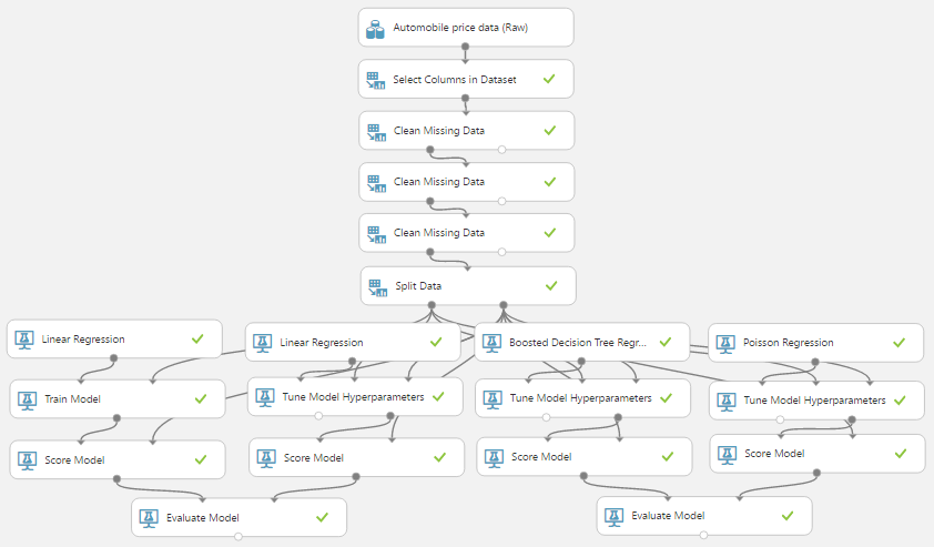
Now that we've created our 70/30 split of the data, let's look at how it fits into the experiment.  We'll start by looking at the two different layouts, Train Model (which is used for Ordinary Least Squares Linear Regression) and Tune Model Hyperparameters (which is used for the other 3 regression algorithms).
Train Model

Tune Model Hyperparameters
We can see that the "Train Model" layout is pretty simple, the Training Set goes into the "Train Model" module and the Testing Set goes into the "Score Model" module.  However, in the "Tune Model Hyperparameters" layout, the Training Set and Testing Set both go in the "Tune Model Hyperparameters" module and the Testing Set also goes into the "Score Model" module.  Let's add all of these together and drop some "Evaluate Model" modules onto the end.
Model Evaluation
Unfortunately, we need two "Evaluate Model" modules because they can only accept two inputs.  Let's take a look at the visulization of the "Evaluate Model" module.
Ordinary Least Squares vs. Online Gradient Descent
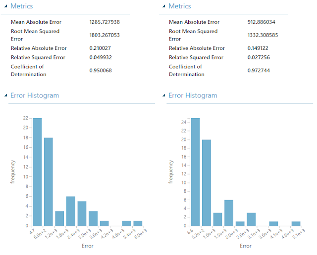
Boosted Decision Tree vs Poisson


Some you may recognize that these visualizations look completely different than those created by the "Evaluate Model" module we used in our previous posts about ROC, Precision, Recall and Lift.  This is because the model evaluation metrics for Regression are completely different than those for Classification.  Looking at the Metrics section, we see that the first four metrics are Mean Absolute Error, Root Mean Squared Error, Relative Absolute Error and Relative Squared Error.  All of these measures tell us how far our predictions deviate from the actual values they are supposed to predict.  We don't generally pay much attention to these, but we do want to minimize these in practice.

The measure we are concerned with is Coefficient of Determination, also known as R Squared.  We've mentioned this metric a number of times during this blog series, but never really described what it tells us.  Basically, R Squared tells us how "good" our  model is at predicting.  Higher values of R Squared are good and smaller values are bad.  It's difficult to determine what's an acceptable value.  Some people say .7 and other people say .8.  If we find anything lower than that, we might want to consider a different technique.  Fortunately for us, the Poisson Regression model has an R Squared of .97, which is extremely good.  As a side note, one of the reasons why we generally don't consider the values of the first four metrics is because they rarely differ from one another.  If R Squared tells you that one model is the best, it's likely that all of the other metrics will tell you the same thing.  R Squared simply has the advantage of being bounded between 0 and 1, which means we can identify not only which model is best, but also if that model is "good enough".

To finalize this evaluation, it seems that the Poisson Regression algorithm is the best model for this data.  This is especially interesting because, in the previous post, we commented on the fact that the Poisson Distribution is not theoretically appropriate for this data.  Given this, it may be a good idea to find an additional set of validation data to confirm our results.  Alas, that's beyond the scope of this experiment.

Hopefully, this discussion has opened your horizons to the possibilities of using Regression to answer some more complex business problems.  Stay tuned for the next post where we'll be talking about Normalizing Features for Regression.  Thanks for reading.  We hope you found this informative.

Brad Llewellyn
Data Scientist
Valorem
@BreakingBI
www.linkedin.com/in/bradllewellyn
llewellyn.wb@gmail.com

Monday, May 1, 2017

Azure Machine Learning: Regression Using Poisson Regression

Today, we're going to continue our walkthrough of Sample 4: Cross Validation for Regression: Auto Imports Dataset.  In the previous posts, we walked through the Initial Data Load, Imputation, Ordinary Least Squares Linear Regression, Online Gradient Descent Linear Regression and Boosted Decision Tree Regression phases of the experiment.
Experiment So Far
Let's refresh our memory on the data set.
Automobile Price Data (Clean) 1

Automobile Price Data (Clean) 2
We can see that this data set contains a bunch of text and numeric data about each vehicle, as well as its price.  The goal of this experiment is to attempt to predict the price of the car based on these factors.  Specifically, we're going to be walking through the Poisson Regression algorithm.  Let's start by talking about Poisson Regression.

Poisson Regression is used to predict values that have a Poisson Distribution, i.e. counts within a given timeframe.  For example, the number of customers that enter a store on a given day may follow a Poisson Distribution.  Given that these values are counts, there are a couple of caveats.  First, the counts cannot be negative. Second, the counts could theoretically extend to infinity.  Finally, the counts must be Whole Numbers.

Just by looking at these three criteria, it may seem like Poisson Regression is theoretically appropriate for this data set.  However, the issue comes when we consider the mathematical underpinning of the Poisson Distribution.  Basically, the Poisson Distribution assumes that each entity being counted operates independently of the other entities.  Back to our earlier example, we assume that each customer entering the store on a given day does so without considering whether the other customers will be going to the store on that day as well.  Comparing this to our vehicle price data, that would be akin to saying that when a car is bought, each dollar independently decides whether it wants to jump out of the buyer's pocket and into the seller's hand.  Obviously, this is a ludicrous notion.  However, we're not theoretical purists and love bending rules (as long as they produce good results).  For us, the true test comes from the validation portion of the experiment, which we'll cover in a later post.  If you want to learn more about Poisson Regression, read this and this.  Let's take a look at the parameters for this module.
Poisson Regression
The Poisson Regression algorithm uses an optimization technique known as Limited Memory Broyden-Fletcher-Goldfarb-Shanno (L-BFGS).  Basically, this technique tries to find the "best" set of parameters to fill in our Poisson Regression equation, which is described in detail here.  In practice, the smaller we make "Optimization Tolerance", the longer the algorithm will take to train and the more accurate the results should be.  This value can be optimized using the "Tune Model Hyperparameters" module.

Without going into too much depth, the "L1 Regularization Weight" and "L2 Regularization Weight" parameters penalize complex models.  If you want to learn more about Regularization, read this and this.  As with "Optimization Tolerance", Azure ML will choose this value for us.

"Memory Size for L-BFGS" specifies the amount of memory allocated to the L-BFGS algorithm.  We can't find much more information about what effect changing this value will have.  Through some testing, we did find that this value had very little impact on our model, regardless of how large or small we made it (the minimum value we could provide is 1).  However, if our data set had an extremely large number of columns, we may find that this parameter becomes more significant.  Once again, we do not have to choose this value ourselves.

The "Random Number Seed" parameter allows us to create reproducible results for presentation/demonstration purposes.  Oddly enough, we'd expect this value to play a role in the L-BFGS algorithm, but it doesn't seem to.  We were unable to find any impact caused by changing this value.

Finally, we can choose to deselect "Allow Unknown Categorical Levels".  When we train our model, we do so using a specific data set known as the training set.  This allows the model to predict based on values it has seen before.  For instance, our model has seen "Num of Doors" values of "two" and "four".  So, what happens if we try to use the model to predict the price for a vehicle with a "Num of Doors" value of "three" or "five"?  If we leave this option selected, then this new vehicle will have its "Num of Doors" value thrown into an "Unknown" category.  This would mean that if we had a vehicle with three doors and another vehicle with five doors, they would both be thrown into the same "Num of Doors" category.  To see exactly how this works, check out of our previous post, Regression Using Linear Regression (Ordinary Least Squares).

The options for the "Create Trainer Mode" parameter are "Single Parameter" and "Parameter Range".  When we choose "Parameter Range", we instead supply a list of values for each parameter and the algorithm will build multiple models based on the lists.  These multiple models must then be whittled down to a single model using the "Tune Model Hyperparameters" module.  This can be really useful if we have a list of candidate models and want to be able to compare them quickly.  However, we don't have a list of candidate models, but that actually makes "Tune Model Hyperparameters" more useful.  We have no idea what the best set of parameters would be for this data.  So, let's use it to choose our parameters for us.
Tune Model Hyperparameters
Tune Model Hyperparameters (Visualization)
We can see that there is very little difference between the top models using Coefficient of Determination, also known as R Squared.  This is a great sign because it means that our model is very robust and we don't have to sweat over choosing the perfect parameters.

On a side note, there is a display issue causing some values for the "Optimization Tolerance" parameter to display as 0 instead of whatever extremely small value they actually are.  This is disappointing as it limits our ability to manually type these values into the "Poisson Regression" module.  One of the outputs from the "Tune Model Hyperparameters" module is the Trained Best Model, whichever model appears at the top of list based on the metric we chose.  This means that we can use this as an input into other modules like "Score Model".  However, it does mean that we cannot use these parameters in conjunction with the "Cross Validate Model" module as that requires an Untrained Model as an input.  Alas, this is not a huge deal because we see that "Optimization Tolerance" does not have a very large effect on the resulting model.
All Regression Models Complete
Hopefully we've laid the groundwork for you to understand Poisson Regression and utilize it in your work.  Stay tuned for the next post where we'll be talking about Regression Model Evaluation.  Thanks for reading.  We hope you found this informative.

Brad Llewellyn
Data Scientist
Valorem
@BreakingBI
www.linkedin.com/in/bradllewellyn
llewellyn.wb@gmail.com