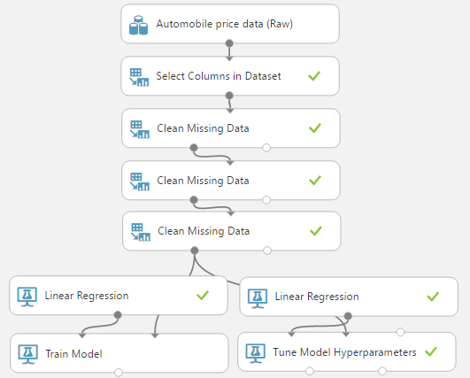
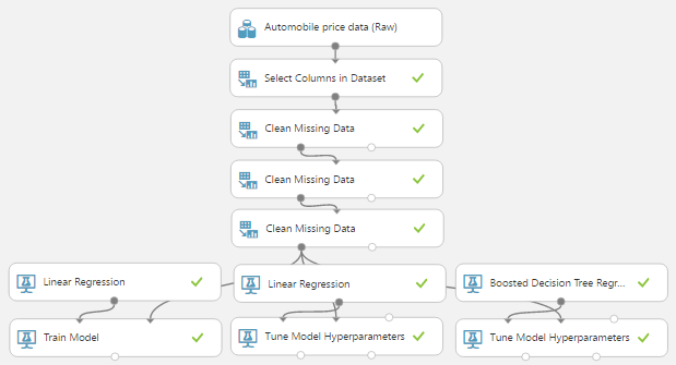
Monday, April 17, 2017

Azure Machine Learning: Regression Using Boosted Decision Tree Regression

Today, we're going to continue our walkthrough of Sample 4: Cross Validation for Regression: Auto Imports Dataset.  In the previous posts, we walked through the Initial Data Load, Imputation, Ordinary Least Squares Linear Regression and Online Gradient Descent Linear Regression phases of the experiment.
Experiment So Far
Let's refresh our memory on the data set.
Automobile Price Data (Clean) 1

Automobile Price Data (Clean) 2
We can see that this data set contains a bunch of text and numeric data about each vehicle, as well as its price.  The goal of this experiment is to attempt to predict the price of the car based on these factors.  Specifically, we're going to be walking through the Boosted Decision Tree Regression algorithm.  Let's start by talking about Decision Tree Regression.
Example Decision Tree
For this example, we used our data set to create a single decision tree with 5 leaves (circled in blue).  Basically, a decision tree is built by choosing the "best" split for each node, then repeating this process until the specified number of leaves is reached.  There's a complex process for choosing the "best" threshold that we won't go into detail on.  You can read more about this process here, here and here.

In our example, we start with the entire dataset.  Then, a single threshold is defined for a single variable that defines the "best" split.  Next, the data is split across the two branches.  On the false side, the algorithm decides that there's not enough data to branch again or the branch would not be "good" enough, so it ends in a leaf.  This means that any records with a value of "Engine Size" > 182 will be assigned a "Predicted Price" of $6,888.41.
Example Decision Tree Predictions
We can see that this is the case by looking at the scored output.  Next, the records with "Engine Size" <= 182 will be passed to the next level and the process will repeated until there are exactly 5 leaves.  Later in this post, we'll see where the 5 came from.

Now, we've talked about "Decision Tree Regression", but what's "Boosted Decision Tree Regression"?  The process of "Boosting" involves creating multiple decision trees, where each decision tree depends on those that were created before it.  For example, assume that we want to build 3 boosted decision trees.  The first decision tree would attempt to predict the price for each record.  The next tree would be calculated using the same algorithm, but instead of predicting price, it would try to predict the difference between the actual price and the price predicted by the previous tree.  This is known as a residual because it is what's "left over" after the tree is built..  For example, if the first tree predicted a price of 10k, but the actual price was 12k, then the second tree would be trying to predict 12k - 10k = 2k instead of the original 12k.  This way, when the algorithm is finished, the predicted price can be calculated simply by running the record through all of the trees, and adding all of the predictions.  However, the process for building the individual trees is more complicated than this example would imply.  You can read about it here and here.  Let's take a look at the "Boosted Decision Tree Regression" module in Azure ML.
Boosted Decision Tree Regression
Some of you may notice that these are the same parameters used in the "Two-Class Boosted Decision Tree" module, which we covered in an earlier post.  Because of the similarity, some of the following descriptions have been lifted from that post.

The "Maximum Number of Leaves per Tree" parameter allows us to set the number of times the tree can split.  It's important to note that splits early in the tree are caused by the most significant predictors, while splits later in the tree are less significant.  This means that the more leaves we have (and therefore more splits), the higher our chance of Overfitting is.  We'll talk more about this in a later post.

The "Minimum Number of Samples per Leaf Node" parameters allows us to set the significance level required for a split to occur.  With this value set at 10, the algorithm will only choose to split (this is known as creating a "new rule") if at least 10 rows, or observations, will be affected.  Increasing this value will lead to broad, stable predictions, while decreasing this value will lead to narrow, precise predictions.

The "Learning Rate" parameter allows us to set how much difference we see from tree to tree.  MSDN describes this quite well as "the learning rate determines how fast or slow the learner converges on the optimal solution. If the step size is too big, you might overshoot the optimal solution. If the step size is too small, training takes longer to converge on the best solution."

The "Random Number Seed" parameter allows us to create reproducible results for presentation/demonstration purposes.  Since this algorithm is not random, this parameter has no impact on this module.

Finally, we can choose to deselect "Allow Unknown Categorical Levels".  When we train our model, we do so using a specific data set known as the training set.  This allows the model to predict based on values it has seen before.  For instance, our model has seen "Num of Doors" values of "two" and "four".  So, what happens if we try to use the model to predict the price for a vehicle with a "Num of Doors" value of "three" or "five"?  If we leave this option selected, then this new vehicle will have its "Num of Doors" value thrown into an "Unknown" category.  This would mean that if we had a vehicle with three doors and another vehicle with five doors, they would both be thrown into the same "Num of Doors" category.  To see exactly how this works, check out of our previous post, Regression Using Linear Regression (Ordinary Least Squares).

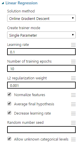
The options for the "Create Trainer Mode" parameter are "Single Parameter" and "Parameter Range".  When we choose "Parameter Range", we instead supply a list of values for each parameter and the algorithm will build multiple models based on the lists.  These multiple models must then be whittled down to a single model using the "Tune Model Hyperparameters" module.  This can be really useful if we have a list of candidate models and want to be able to compare them quickly.  However, we don't have a list of candidate models.  Strangely, that actually makes "Tune Model Hyperparameters" more useful.  We have no idea what the best set of parameters would be for this data.  So, let's use it to choose our parameters for us.
Tune Model Hyperparameters
Tune Model Hyperparameters (Visualization)
We can see that the "Tune Model Hyperparameters" module will test quite a few different models in order to determine the best combination of parameters.  In this case, it found that a set of 44 trees with 4 leaves, a significance level of 2 records per leaf and a learning rate of .135 has the highest Coefficient of Determination, also known as R Squared.
OLS/OGD Linear Regression and Boosted Decision Tree Regression
Now, our experiment contains 3 different regression methods for predicting the price of a vehicle.  Hopefully, this post opened the door for you to utilize Boosted Decision Tree Regression in your own work.  Stay tuned for our next post where we'll talk about Poisson Regression.  Thanks for reading.  We hope you found this informative.

Brad Llewellyn
Data Scientist
Valorem
@BreakingBI
www.linkedin.com/in/bradllewellyn
llewellyn.wb@gmail.com

Monday, April 3, 2017

Azure Machine Learning: Regression Using Linear Regression (Online Gradient Descent)

Today, we're going to continue our walkthrough of Sample 4: Cross Validation for Regression: Auto Imports Dataset.  In the previous posts, we walked through the Initial Data Load, Imputation and Ordinary Least Squares Linear Regression phases of the experiment.
Experiment So Far
Let's refresh our memory on the data set.
Automobile Price Data (Clean) 1

Automobile Price Data (Clean) 2
We can see that this data set contains a bunch of text and numeric data about each vehicle, as well as its price.  The goal of this experiment is to attempt to predict the price of the car based on these factors.  Specifically, we're going to be walking through the Online Gradient Descent algorithm for Linear Regression.  Let's take a look at the parameters.
Linear Regression (OGD)
The "Online Gradient Descent" algorithm creates multiple regression models based on the parameters we provide.  The goal of these regression models is to find the model that fits the data "best", i.e. has the smallest "loss" according a particular loss function.  As with all of the iterative procedures, we trade additional training time and the possibility of getting "stuck" in local extrema in exchange for the change of finding a better solution.  You can read more about OGD here.
Gradient
Here's a visual representation of a gradient that we pulled from Wikipedia.  This valley represents the "loss" or "error" of our model.  Lower "loss" means a better model.  The goal of the OGD algorithm is find the bottom of the valley in the picture.  Basically, a starting point is randomly assigned and the algorithm simply tries to keep going downhill by building new models.  If it keeps going downhill, it will eventually reach the bottom of the valley.  However, things get much more complicated when you have multiple valleys (what if you get to the bottom of one valley, but there's an even deeper valley next to it?).  We'll touch on this in a minute.  Let's walk through the parameters.

"Learning Rate" is also known as "Step Size".  As the algorithm is trying to go downhill, it needs to know how far to move each time.  This is what "Learning Rate" represents.  A smaller step size would mean that we are more likely to find the bottom of the valley, but it also means that if we stuck in a valley that isn't the deepest, we may not be able to get out.  Conversely, a larger step size would mean that we can more easily find the deepest valley, but may not be able to find the bottom of it.  Fortunately, we can let Azure ML choose this value for us based on our data.

"Number of Training Epochs" defines how many times the algorithm will go through this learning process.  Obviously, the larger the number of iterations, the longer the training process will take.  Also, larger values could potentially lead to overfitting.  As with the other parameters, we don't have to choose this ourselves.

Without going into too much depth, the "L2 Regularization Weight" parameter penalizes complex models in favor of simpler ones.  Fortunately, there's a way that Azure ML will choose this value for us.  So, we don't need to worry too much about it.  If you want to learn more about Regularization, read this and this.

According to MSDN, "Normalize Features" allows us to "indicate that instances should be normalized".  We're not quite sure what this is supposed to mean.  There is a concept in regression of normalizing, also known as standardizing, the inputs.  However, we did some testing and were not able to find a situation where this feature had any effect on the results.  Please let us know in the comments if you know of one.

"Average Final Hypothesis" is much more complicated.  Here's the description from MSDN:
In regression models, hypothesis testing means using some statistic to evaluate the probability of the null hypothesis, which states that there is no linear correlation between a dependent and independent variable. 
In many regression problems, you must test a hypothesis involving more than one variable. This option, which is selected by default, tests a combination of the parameters where two or more parameters are involved.
This seems to imply that utilizing the "Average Final Hypothesis" option takes into account the interactions between factors, instead of assuming they are independent.  Interestingly,  deselecting this option seems to generally produce better models.  However, it also has an unwritten size limit.  If we deselect this option and try to train the model using too many rows or columns, it will throw an error.  Therefore, we can say that deselecting this option is extremely useful in some cases.  We'll have to try it case-by-case to decide when it is appropriate and when it is not.

The "Decrease Learning Rate" option allows Azure ML to decrease the Learning Rate (aka Step Size) as the number of iterations increases.  This allows us to hone in on an even better model by allowing us to find the tip of the valley.  However, reducing the learning rate also increases the chances that we get stuck in a local minima (one of the shallow valleys).  Deselecting this option is susceptible to the same size limitation as "Average Final Hypothesis", but doesn't seem to have the same positive impact.  Unless we can find a good reason, let's leave this option selected for the time being.

Choosing a value for "Random Number Seed" defines our starting point and allows us to create reproducible results in case we need to use them for demonstrations or presentations.  If we don't provided a value for this parameter, one will be randomly generated.

Finally, we can choose to deselect "Allow Unknown Categorical Levels".  When we train our model, we do so using a specific data set known as the training set.  This allows the model to predict based on values it has seen before.  For instance, our model has seen "Num of Doors" values of "two" and "four".  So, what happens if we try to use the model to predict the price for a vehicle with a "Num of Doors" value of "three" or "five"?  If we leave this option selected, then this new vehicle will have its "Num of Doors" value thrown into an "Unknown" category.  This would mean that if we had a vehicle with three doors and another vehicle with five doors, they would both be thrown into the same "Num of Doors" category.  To see an example of this, read our previous post.

Now that we've walked through all of the parameters, we can use the "Tune Model Hyperparameters" module to choose them for us.  However, it will only choose values for "Learning Rate", "Number of Epochs" and "L2 Regularization Weight".  Since we also found that "Average Final Hypothesis" was significant, we should create two separate streams, one with this option selected and one without.  For an explanation of how "Tune Model Hyperparameters" works, read one our previous posts.
Tune Model Hyperparameters

Tune Model Hyperparameters (Visualization) (Average Final Hypothesis)

Tune Model Hyperparameters (Visualization) (No Average Final Hypothesis)
The first thing we noticed is that when we deselect the "Average Final Hypothesis" option, we lose 6 rows because of the size limit.  Certain combinations of parameters caused the model to fail.  Fortunately, the "Tune Model Hyperparameters" module is smart enough to throw them out.  In fact, not all 14 of the remaining rows are valid.  For instance, the last row has a Coefficient of Determination (R Squared) of -5e51.  That's -5 followed by 51 zeroes.  That's obviously an error considering that R Squared is supposed to be bounded between 0 and 1.

Also, it's important to note that the best model with "Average Final Hypothesis" has an R squared of .678 compared to an R squared of .769 without.  This is what we meant when we said that disabling the option seems to produce better results.  Unfortunately, our lack of familiarity with what the parameter actually does means that we're not sure if this result is valid or not.  The best we can do is assume that it is.  If you have any information on this, please let us know.
OLS and OGD Linear Regression
So far in this experiment, we've covered the basics of Data Import and Cleansing, Ordinary Least Squares Linear Regression and Online Gradient Descent Linear Regression.  However, that's just the tip of the iceberg.  Stay tuned for the next post where we'll be covering Boosted Decision Tree Regression.  Thanks for reading.  We hope you found this informative.

Brad Llewellyn
Data Scientist
Valorem
@BreakingBI
www.linkedin.com/in/bradllewellyn
llewellyn.wb@gmail.com