|
| Estimate |
 |
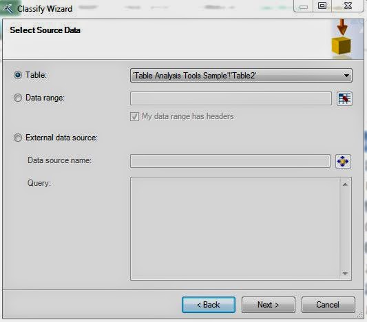
| Select Data Source |
 |
| Column Selection |
In a combination decision tree/regression model like this, there are two types of predictors, Regressors and Categories. As a simple example, let's try to predict Income using Age and Region. The model itself looks like
Income = C1 * V1 + C2 * V2 + ...
where the C's are fixed values determined by the model and the V's are variables that come from the data. When you set a value as a Regressor, Age in our example, then Age is thrown directly in as a variable, like so
Income = C1 * Age + C2 * V2 + ...
However, Region isn't a numeric variable at all, how would you put it in this formula at all? There is a technique called Dummy Variables. You can read about it here. Basically, you create a variable for each value that the variable can take. For instance, Region can be "North America", "Europe", and "Pacific". So, you would create a 1/0 variable for each value of Region. Mathematically, you can actually leave one of the variables out entirely and it won't matter, but we won't go that far. Read the article if you're truly interested. So, our model would become
Income = C1 * Age + C2 * [Region = North America] + C3 * [Region = Europe] + C4 * [Region = Pacific]
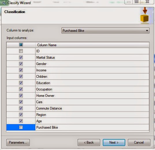
In summary, any value that you want treated as a number should be a regressor and any value you want treated as a category should just be an input. However, this algorithm in particular looks at things in a slightly different way. The Categories are used to create the nodes in the tree and the Regressors are used in the regression equation. You'll see what we mean in a minute. Let's look at our columns again.
 |
| Column Selection |
As you can see, we set all of the numeric variables as regressors and the rest of the variables as inputs. As usual, we don't include the ID or the value we're trying to predict. Let's check out the parameters.
 |
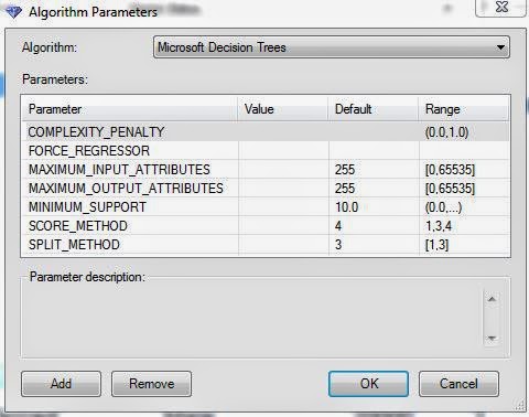
| Parameters |
Remember how we said this is the same algorithm we used for Decision Trees? Well that means that is also has the same parameters. They can be very useful if you're trying to tweak the model to fit your needs. We won't mess with it for now. Let's keep moving.
 |
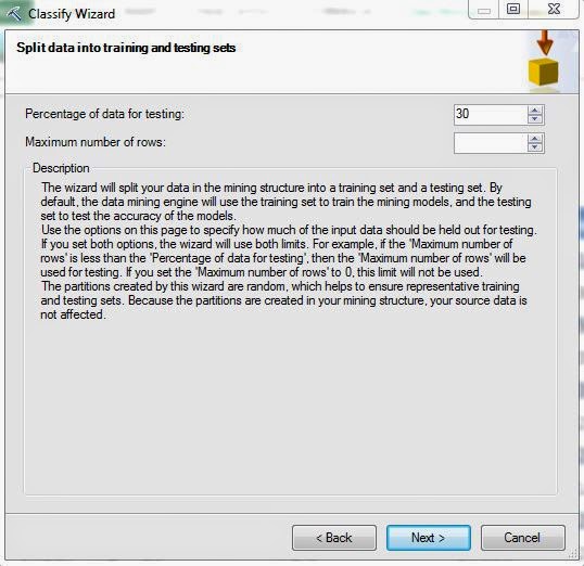
| Training Set Selection |
As with all of the Data Mining Tools, we need to specify the size of the Training set. We'll keep the default 70%.
 |
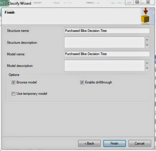
| Model Creation |
Finally, we have to create a structure and a model to store our work. These are housed directly on the Analysis Services server and can be recalled later if you wish. Let's check out the results.
 |
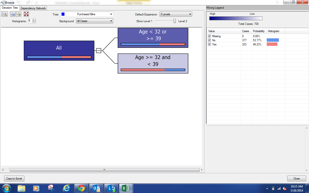
| Browse |
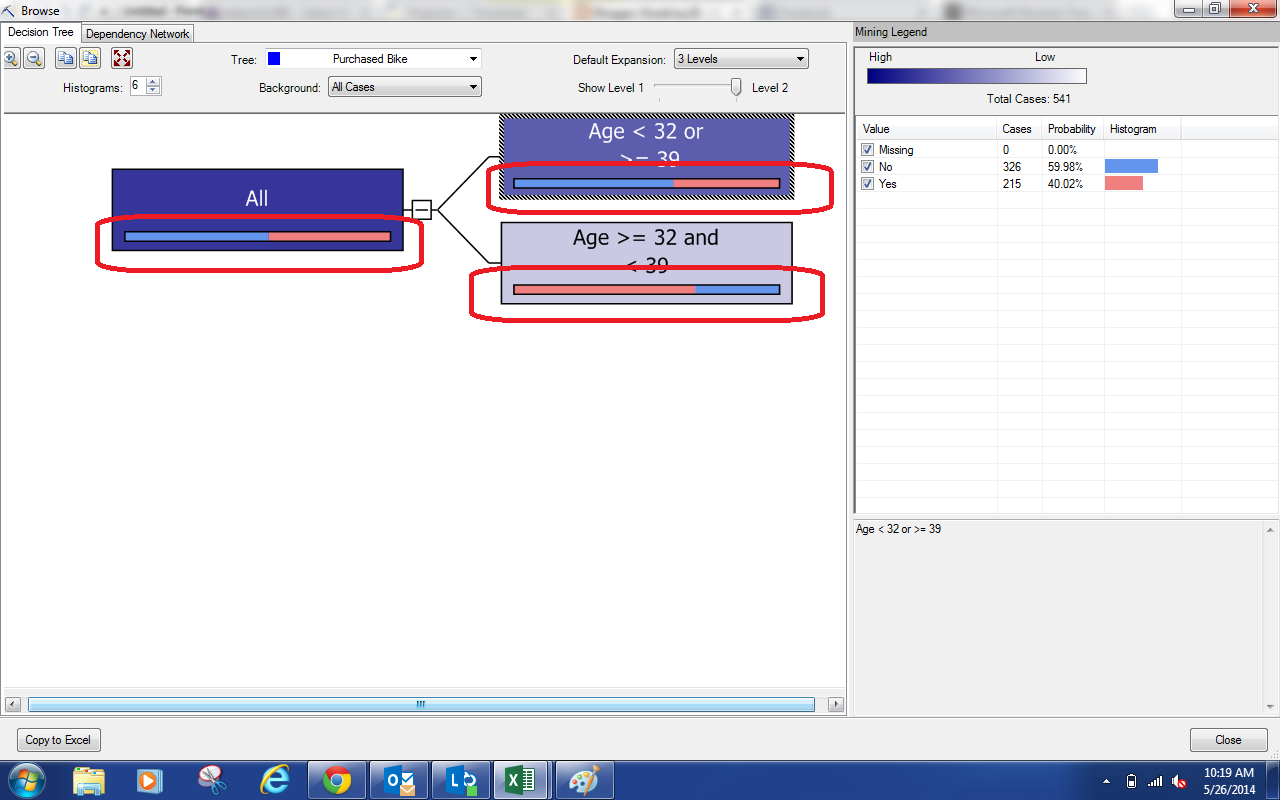
We get a pretty big tree on our first try. If you're not familiar with the tree diagram, you can check out Part 15. There are a couple of differences here. Let's highlight them.
 |
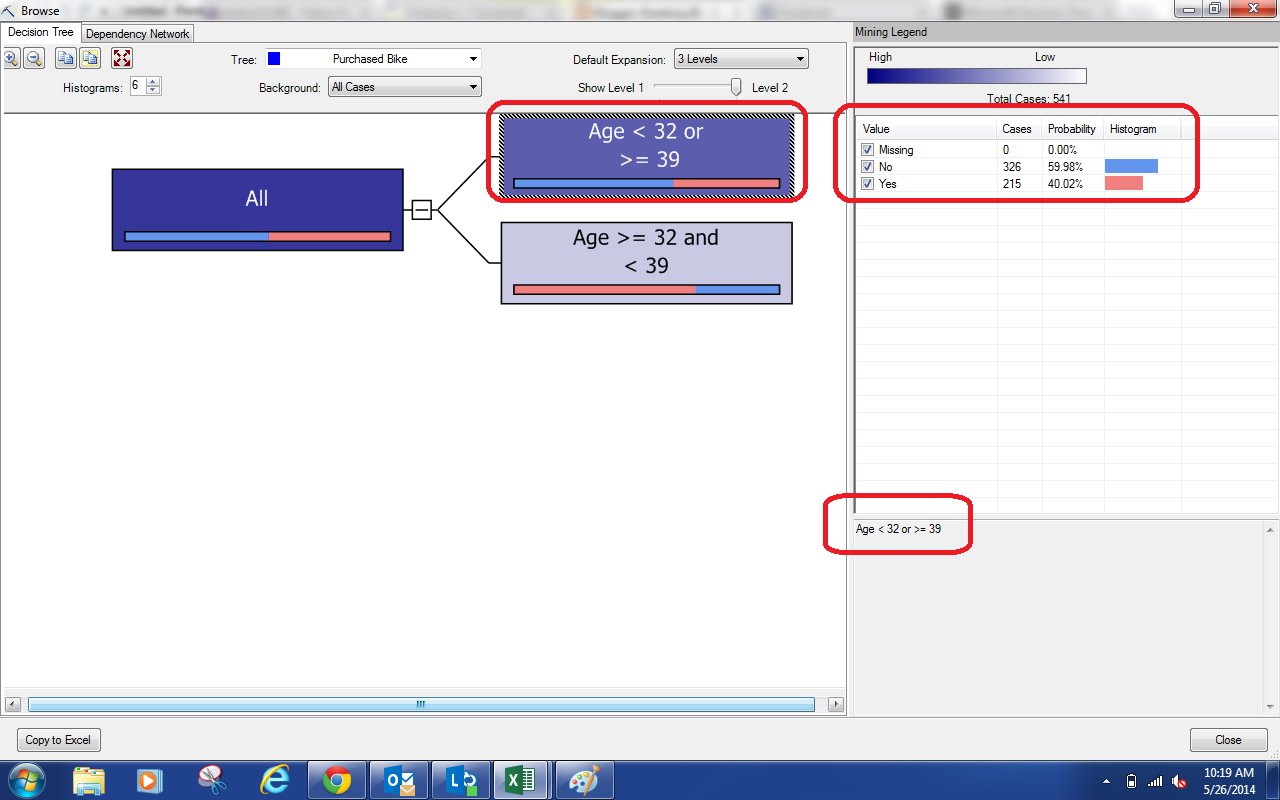
| Nodes |
Just like the previous Decision Trees, each node can branch into further nodes. However, notice the bars that we've highlighted in red? Each node represents a chunk of our data set. This diamond represents the distribution of the Incomes within the node. The further to the left or right the diamond is tells us where the average Income falls within this chunk. We see that all of these nodes have low incomes because they are far to the left. The wider the diamond is, the more spread out the incomes are, meaning that our predictions are likely to be less accurate. Despite being low incomes, these diamonds are all very small, which means we can be confident in the predictions. Let's look at another piece of diagram.
 |
| Coefficients |
Remember the C's and V's we saw earlier in our formula. The C's are the coefficients and are represented by the values in brown. The V's are the variables and are represented by the values in red. Combining these two allows us to create the formula that you can see at the bottom of the screen. We won't go into explaining this formula more than we already have. It's interesting to note that each node gets its own formula. Just remember this, the categories create the nodes and the regressors create the formula. Let's move on.
 |
| Dependency Network |
This algorithm has Dependency Networks just like the last one. If you're unfamiliar with Dependency Networks, check out Part 16.
By now, you should be seeing some use for these algorithms. Even if you're not, there's still much more to come. You might be asking "A pretty picture is great; but, how do I get the predictions into the data?" Unfortunately, that's a more involved task for another post. We'll restate it again for everyone to hear, "If you want the simple things done easily, check out the Table Analysis tools. But, if you want to do the cool stuff and really push Data Mining to its limits, you need to learn to use the Data Mining tools." Keep an eye out for our next post, where we'll be discussing Clustering. Thanks for reading. We hope you found this informative.
Brad Llewellyn
Director, Consumer Sciences
Consumer Orbit
llewellyn.wb@gmail.com
Director, Consumer Sciences
Consumer Orbit
llewellyn.wb@gmail.com
http://www.linkedin.com/in/bradllewellyn


.png)


.png)
.png)
.png)


.png)
.png)