Monday, January 28, 2019

Data Science in Power BI: Stream Analytics

Today, we're going to talk about Stream Analytics within Power BI.  If you haven't read the earlier posts in this series, Introduction, Getting Started with R Scripts, Clustering, Time Series Decomposition, Forecasting, Correlations, Custom R Visuals, R Scripts in Query Editor, Python and Azure Machine Learning Studio, they may provide some useful context.  You can find the files from this post in our GitHub Repository.  Let's move on to the core of this post, Stream Analytics.

Stream Analytics is an Azure service for processing streaming data from Event Hub, IoT Hub or Blob Storage using a familiar SQL-like language known as "Stream Analytics Query Language".  This language allows us to interpret JSON, Avro and CSV data in a way that will be very familiar to SQL developers.  It is also possible to aggregate data using varying types of time windows, as well as join data streams to each other or to other reference sets.  Finally, the resulting data stream can be output to a number different destinations, including Azure SQL Database, Azure Cosmos DB and Power BI.

We understand that streaming data isn't typically considered "Data Science" by itself.  However, it's are often associated and setting up this background now opens up some cool applications in later posts.  For this post, we'll cover how to sink streaming data to Power BI using Stream Analytics.

The previous posts in this series used Power BI Desktop for all of the showcases.  This post will be slightly different in that we will leverage the Power BI Service instead.  The Power BI Service is a collaborative web interface that has most of the same reporting capabilities as Power BI Desktop, but lacks the ability to model data at the time of writing.  However, we have heard whispers that data modeling capabilities may be coming to the service at some point.  The Power BI Service is also the standard method for sharing datasets, reports and dashboards across organizations.  For more information on the Power BI Service, read this.

In order to leverage Stream Analytics, we obviously need to start by creating a source of streaming data.  In order to do this, we'll leverage some sneaky functionality with Azure SQL Database and Azure Data Factory (ADF).  Basically, we want to trigger an ADF Pipeline every minute that pulls between 1 and 5 random records from our database, placing these records in Blob Storage.  We'll pretend that this is our "stream".  Stream Analytics will then pick up these records, process them and sink them to Power BI.  The flow should look like this:
Customer Stream
This is going to be an extension of the "Customers" tables we created in the previous post.  We'll start by creating a SQL Stored Procedure called "Customers_ADFSource" that pulls between 1 and 5 random records from the "Customers_New" table.

<CODE START>

CREATE PROCEDURE Customers_ADFSource AS
BEGIN

DECLARE @records INT = ( SELECT CEILING( RAND() * 4 ) + 1 )

BEGIN
WITH T AS (
SELECT
ROW_NUMBER() OVER ( ORDER BY NEWID() )AS [rownumber]
,NEWID() AS [customerid]
,[age]
,[workclass]
,[fnlwgt]
,[education]
,[education-num]
,[marital-status]
,[occupation]
,[relationship]
,[race]
,[sex]
,[capital-gain]
,[capital-loss]
,[hours-per-week]
,[native-country]
FROM Customers_New
)

SELECT
[customerid]
,[age]
,[workclass]
,[fnlwgt]
,[education]
,[education-num]
,[marital-status]
,[occupation]
,[relationship]
,[race]
,[sex]
,[capital-gain]
,[capital-loss]
,[hours-per-week]
,[native-country]
FROM T
WHERE [rownumber] < @records
END

END

<CODE END>

EDIT: After writing this, we later found that this could also be achieved by using something similar to "SELECT TOP (@records) * FROM [Customers_New]".  The parentheses are extremely important as this will not work without them.
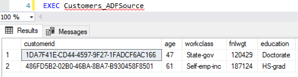

Customers_ADFSource
Notice that we aren't bringing over the "Income" column.  This will become important in the new post.  We're also assigning new GUIDs to each record so that we can pretend that these are always new customers, even if they happen to have the exact same attributes as a previous customer.

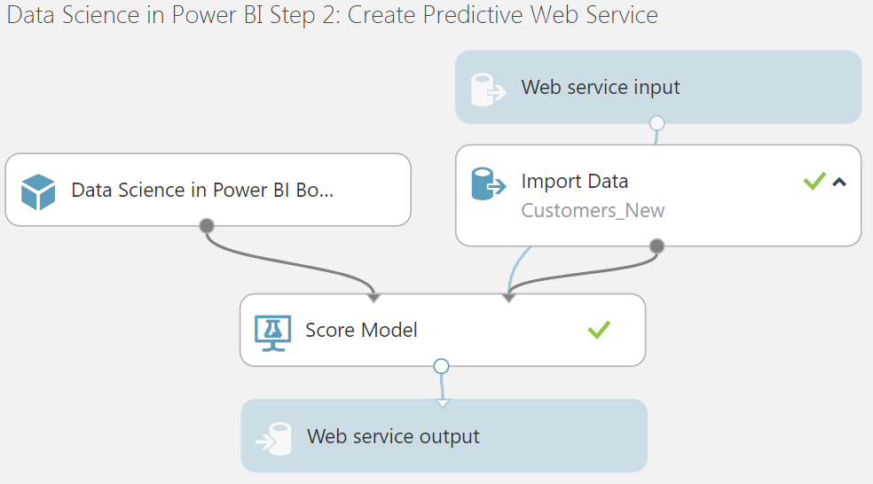
Next, we want to create an ADF Pipeline that executes the "Customers_ADFSource" Stored Procedure and loads the data into the "customerssasource" Blob Container.  Showcasing this would take way too many screenshots for us to add here.  Feel free to take it on as an exercise for yourselves, as it's not terribly complicated once you have the SQL Stored Procedure created.
customerssasource
<OUTPUT START>

{"customerid":"5c83d080-d6ba-478f-b5f0-a511cf3dee48","age":56,"workclass":"Private","fnlwgt":205735,"education":"1st-4th","education-num":2,"marital-status":"Separated","occupation":"Machine-op-inspct","relationship":"Unmarried","race":"White","sex":"Male","capital-gain":0,"capital-loss":0,"hours-per-week":40,"native-country":"United-States"}

{"customerid":"6b68d988-ff75-4f63-b278-39d0cf066e96","age":25,"workclass":"Private","fnlwgt":194897,"education":"HS-grad","education-num":9,"marital-status":"Never-married","occupation":"Sales","relationship":"Own-child","race":"Amer-Indian-Eskimo","sex":"Male","capital-gain":6849,"capital-loss":0,"hours-per-week":40,"native-country":"United-States"}


<OUTPUT END>

We see that the ADF pipeline is placing one file containing between 1 and 5 customer records in the blob container every minute.  Now that we have emulated a stream of Customer data, let's use Stream Analytics to process this stream and sink it to Power BI.  We start by creating an empty Stream Analytics job.  This is so simple that we won't cover it in this post.
After it's created, we see that we have four different components in the "Job Topology" section of the Stream Analytics blade.  We'll start by creating an input that reads data from our Blob Container.
Create Blob Input
CustomersSASource (SA)


We have called this input "Customers_SASource".  Next, we want to create a stream output that sinks to Power BI.
Create Power BI Output
CustomersStream
Now that we have an input and an output, we need to create a query.  As we mentioned earlier, the Stream Analytics Query Language is a SQL-like language that makes it relatively painless to access Stream Analytics inputs that may be stored in semi-structured formats, such as CSV, JSON and AVRO.  In our case, we'll just use "SELECT *" to pass through all of the data.
Query
While writing this, we discovered that Stream Analytics will allow us to create input and outputs with underscores ( _ ) in the names, but the Query Editor considers them to syntax errors.  This is an odd compatibility issue that should be noted.

Now, the last step is to go to the Power BI Portal and navigate to the workspace where we stored our dataset.
My Workspace
By clicking on the "CustomersStream" dataset, we can create a simple report that shows us the total number of Customers that are streaming into our dataset.
CustomersStreamReport
While this functionality is pretty cool, the Power BI Service still has a long way to go in this respect.  Additional effort is needed to make the report always show a relative time frame, like the last 30 minutes.  Reports also don't seem to automatically refresh themselves in any way.  When we wanted to see the most recent data from the stream, we had to manually refresh this report.  This issue also occurs if we pin a live report to a dashboard.  However, we found that individually pinning the visuals to the dashboard allows them automatically update.
CustomersStreamDashboard
The left side of the dashboard shows a live report tile, while the right side of the dashboard shows a set of pinned visuals.  As for our "last 30 minutes" issue mentioned earlier, we can work around this by leveraging Custom Streaming Dashboard Tiles.  These tiles provide a very limited set of functionality for viewing live streaming data from a dashboard.  You can read more about them here.
Custom Streaming Dashboard Tiles
Hopefully, this post enlightened you to some of the ways that Power BI can be used to consume streaming data.  The use cases for streaming data are constantly evolving, as there seem to be new opportunities every day.  Stay tuned for the next post where we'll add some Azure Machine Learning Studio integration into our Stream Analytics job.  Thanks for reading.  We hope you found this informative.

Brad Llewellyn
Service Engineer - FastTrack for Azure
Microsoft
@BreakingBI
www.linkedin.com/in/bradllewellyn
llewellyn.wb@gmail.com

Monday, January 7, 2019

Data Science in Power BI: Azure Machine Learning Studio

Today, we're going to talk about Azure Machine Learning Studio within Power BI.  If you haven't read the earlier posts in this series, Introduction, Getting Started with R Scripts, Clustering, Time Series Decomposition, Forecasting, Correlations, Custom R Visuals, R Scripts in Query Editor and Python, they may provide some useful context.  You can find the files from this post in our GitHub Repository.  Let's move on to the core of this post, Azure Machine Learning Studio.

Azure Machine Learning Studio is a tool that we have talked about extensively on this blog.  It allows us to create advanced analytic and predictive modeling experiments using an intuitive, drag-and-drop interface.  It also allows us to easily productionalize our predictive models by using Azure Machine Learning Studio APIs.  Here are links to the first posts in two different series that cover these topics, Azure Machine Learning: Getting Started and Azure Machine Learning in Practice: Fraud Detection.

In this post, we're going to use an Azure Machine Learning Studio dataset that we've seen in a number of posts, as well as our presentations, Azure Machine Learning Studio: Making Data Science Easy(er) and Azure Machine Learning Studio: Four Tips from the Pros.  This is the Adult Census Income Binary Classification Dataset.  Our goal will be to predict the customer's income based on a number of demographic features.

Since we're going to be using this dataset in Azure Machine Learning Studio and Power BI, the easiest option is to put it in an Azure SQL Database and let both of them query it from there.  Before we do that, we want to split the data into two different sets, a training set for building the model and a testing set for testing the results.  We've talked about this technique a number of times on this blog.  Here's one example.  Fortunately, this is quite easy to do in Azure Machine Learning Studio using the "Split Data" module.
Create Testing and Training Sets
We also need to create the tables in Azure SQL Database to store the data.  Here's the code we used for that.

<CODE START>

CREATE TABLE Customers (
age INT
,workclass NVARCHAR(255)
,fnlwgt INT
,education NVARCHAR(255)
,[education-num] INT
,[marital-status] NVARCHAR(255)
,occupation NVARCHAR(255)
,relationship NVARCHAR(255)
,race NVARCHAR(255)
,sex NVARCHAR(255)
,[capital-gain] INT
,[capital-loss] INT
,[hours-per-week] INT
,[native-country] NVARCHAR(255)
,income NVARCHAR(255)
)

CREATE TABLE Customers_New (
age INT
,workclass NVARCHAR(255)
,fnlwgt INT
,education NVARCHAR(255)
,[education-num] INT
,[marital-status] NVARCHAR(255)
,occupation NVARCHAR(255)
,relationship NVARCHAR(255)
,race NVARCHAR(255)
,sex NVARCHAR(255)
,[capital-gain] INT
,[capital-loss] INT
,[hours-per-week] INT
,[native-country] NVARCHAR(255)
,income NVARCHAR(255)

)

<CODE END>

After loading the data to the tables, we confirm the data's there and can move on to creating the predictive model.
Check Record Counts
Next, we want to create and evaluate our model for predicting "income".
Create Predictive Model
Evaluation Results
We can see that our model has an Accuracy of 86.7% and an AUC of 92.2%.  Let's assume that this is good enough for us to publish and use in our Power BI reports.  The next step is to publish this as a web service.  We've covered this approach in a previous post.
Create Predictive Web Service
Web Service Deployed


Now that we have the web service deployed to Azure, we need to be able to call this from Power BI.  To do this, we could use either R or Python.  Since Python is still in preview at the time of writing, we'll use R.  Fortunately, the Azure Machine Learning Web Services portal provides the code for us.  All we have to do is navigate to the "Consume" tab and select "Request-Response -> R".
Consume
Request-Response R Code


Here's the code that it provides.

<CODE START>

library("RCurl")
library("rjson")

# Accept SSL certificates issued by public Certificate Authorities
options(RCurlOptions = list(cainfo = system.file("CurlSSL", "cacert.pem", package = "RCurl")))

h = basicTextGatherer()
hdr = basicHeaderGatherer()

req =  list(
    Inputs = list(
            "input1"= list(
                list(
                        'id' = "1",
                        'age' = "1",
                        'workclass' = "",
                        'fnlwgt' = "1",
                        'education' = "",
                        'education-num' = "1",
                        'marital-status' = "",
                        'occupation' = "",
                        'relationship' = "",
                        'race' = "",
                        'sex' = "",
                        'capital-gain' = "1",
                        'capital-loss' = "1",
                        'hours-per-week' = "1",
                        'native-country' = "",
                        'income' = ""
                    )
            )
        ),
        GlobalParameters = setNames(fromJSON('{}'), character(0))
)

body = enc2utf8(toJSON(req))
api_key = "abc123" # Replace this with the API key for the web service
authz_hdr = paste('Bearer', api_key, sep=' ')

h$reset()
curlPerform(url = "https://ussouthcentral.services.azureml.net/subscriptions/143cebb47ba243ec9422da9787ff546b/services/2be5b160bdca49e4aa580f21795ff1e5/execute?api-version=2.0&format=swagger",
httpheader=c('Content-Type' = "application/json", 'Authorization' = authz_hdr),
postfields=body,
writefunction = h$update,
headerfunction = hdr$update,
verbose = TRUE
)

headers = hdr$value()
httpStatus = headers["status"]
if (httpStatus >= 400)
{
print(paste("The request failed with status code:", httpStatus, sep=" "))

# Print the headers - they include the requert ID and the timestamp, which are useful for debugging the failure
print(headers)
}

print("Result:")
result = h$value()

print(fromJSON(result))

<CODE END>

Since this code uses a hard-coded list of 1's and empty strings.  We can directly test this in RStudio without needing to use it in Power BI yet.  In order to use this code, we need to install the "RCurl" and "rjson" packages.  RCurl allows us to execute HTTP Requests against web service endpoints, while rjson allows us to create and parse the json payloads used by the web service.  We also need to provide our API Key on the following line:

api_key = "abc123" # Replace this with the API key for the web service

The API Key can be found on the "Consume" tab of the Azure Machine Learning Web Services Portal.

The final output from the R code is as follows:

<OUTPUT START>

$Results
$Results$output1
$Results$output1[[1]]
$Results$output1[[1]]$id
[1] "1"

$Results$output1[[1]]$age
[1] "1"

$Results$output1[[1]]$workclass
NULL

$Results$output1[[1]]$fnlwgt
[1] "1"

$Results$output1[[1]]$education
NULL

$Results$output1[[1]]$`education-num`
[1] "1"

$Results$output1[[1]]$`marital-status`
NULL

$Results$output1[[1]]$occupation
NULL

$Results$output1[[1]]$relationship
NULL

$Results$output1[[1]]$race
NULL

$Results$output1[[1]]$sex
NULL

$Results$output1[[1]]$`capital-gain`
[1] "1"

$Results$output1[[1]]$`capital-loss`
[1] "1"

$Results$output1[[1]]$`hours-per-week`
[1] "1"

$Results$output1[[1]]$`native-country`
NULL

$Results$output1[[1]]$income
NULL

$Results$output1[[1]]$`Scored Labels`
NULL

$Results$output1[[1]]$`Scored Probabilities`

NULL

<OUTPUT END>

Since we passed a useless test record to the web service, we got NULL responses for the "Scored Labels" and "Scored Probabilities" fields.  This will not be the case once we start passing legitimate records.

Unfortunately, this code still isn't quite ready for Power BI.  The output we just showed is in the form of a nested set of lists.  The Power BI Query Editor needs this data to be in a data frame.  We start by accessing the inner list containing the actual values.
Result List
<CODE START>

result.list <- fromJSON(result)$Results$output1[[1]]
result.list

<CODE END>

This code is relatively simple.  From right-to-left (inner-to-outer), this code accesses the first element in the "output1" list contained within the "Results" list contained within the list returned by parsing the JSON in the "result" variable.  Now, let's try to cast this to a data frame.
Result Data Frame (Naive Attempt)
Unfortunately, we get an error saying that the objects in the list are not of the same length.  It seems to have an issue with the fact that some of these objects are NULL.  In R, "NULL" is not a object.  However, R also has an object that represents no value.  This object is called "NA".  So, we need to change all of the NULL "values" in our list to NAs before we can create our data frame.
Result List (with NAs)
<CODE START>

result.list[sapply(result.list, is.null)] <- NA
result.list

<CODE END>

This function enters an "NA" value into each element of the list that contains a NULL "value".  Now, we can cast this to a data frame with no issues.
Result Data Frame
<CODE START>

result.df <- data.frame(result.list)
result.df

<CODE END>

Now that our code returns a data frame, we need to use it in Power BI.  In order to do that, let's switch over to Power BI and connect to the "Customers_New" table in our Azure SQL Database.
Customers_New
We have the option of using this web service in two ways.  First, we could use it as part of a Custom R Visual, which we've talked about in a previous post.  This would allow us to utilize the predictive model based on filters and user input.  This is especially helpful for scenarios like clustering and time series analysis where you want to be able to see the effects of filtering certain items.

Second, we could use an R Script in the Query Editor, which we've also talked about in a previous post.  This would allow us to utilize the web service only during model processing and store the values within the data model itself for aggregation and manipulation as we see fit.

Before we can successfully run our code in the Power BI Query Editor, we need to make a few alterations to our code.  We start by replacing the manually-created "reg" list with one that we create from our input dataset, which Power BI conveniently calls "dataset".

<CODE START>

req =  list(
  Inputs = list(
    input1 = setNames(lapply(split(dataset, seq(nrow(dataset))), FUN = as.list), NULL)
  ),
  GlobalParameters = setNames(fromJSON('{}'), character(0))

)

<CODE END>

It's important to note that the syntax here is extremely important.  While it is possible to put "Inputs" and "input1" inside single-quotes, this changes the metadata of the list structure and could cause the web service call to fail.  This was a particularly frustrating issue to debug.

As for the code, we start by using the "split()" function to split the "dataset" dataframe into a list such that each element in the list is a row from the original dataframe.  The "seq(nrow(dataset))" provides the mapping to ensure that each element in the dataframe is split to the correct element in the list.

Then, we use the "lapply()" function to apply the "as.list()" function to each element in the list.  This turns each dataframe in the list into a nested list containing the data from that record of the dataframe.  Finally, we need to remove the names from the outer list using the "setNames()" function with the "NULL" parameter.  This nested listed is then assigned as a nested list called "input1" within a list called "Inputs" within another list called "req".  This creates the nested structure required by the web service.

Next, we rewrite the error-handling at the end to send an error dataframe to Power BI if an error occurs.

<CODE START>

if (httpStatus >= 400)
{
   result.error <- data.frame("Error")
}

print("Result:")
result = h$value()

print(fromJSON(result))

<CODE END>

We accomplished this by using the "data.frame()" function to create a basic dataframe called "result.error" that contains a single record, "Error".

Next, we need to alter the code to output the final result as a data frame, instead of simply printing the JSON.

<CODE START>

if (httpStatus >= 400){
  result.error <- data.frame("Error")
}else{
  result.json = h$value()
  result.list = fromJSON(result.json)$Results$output1
  result.list.final <- lapply(result.list, FUN = function(x) lapply(x, FUN = function(y) if( is.null(y) ){y <- NA}else{y <- y}))
  result.df <- data.frame(do.call(rbind.data.frame, result.list.final))

}

<CODE END>

We aren't afraid to admit that getting this right took us some time.  We start by assigning the JSON output from the web service to the "result.json" object.  Then, we use the "fromJSON" function to parse the results and save them as a list called "result.list".  There's one caveat here.  If the web service returns any NULL values, then this list will contain those NULL values.  As we mentioned earlier in this post, NULL in R means that the object itself does not exist, which causes errors later on.  Instead, we need to assign NA to these values.  We accomplished this by nesting an if statement within two levels of "lapply" functions.  Finally, we can cast our list as a data frame using the "data.frame", "do.call" and "rbind.data.frame" functions.

Here's the full script.

<CODE START>

library("RCurl")
library("rjson")

# Accept SSL certificates issued by public Certificate Authorities
options(RCurlOptions = list(cainfo = system.file("CurlSSL", "cacert.pem", package = "RCurl")))

h = basicTextGatherer()
hdr = basicHeaderGatherer()

req =  list(
  Inputs = list(
    input1 = setNames(lapply(split(dataset, seq(nrow(dataset))), FUN = as.list), NULL)
  ),
  GlobalParameters = setNames(fromJSON('{}'), character(0))
)

body = enc2utf8(toJSON(req))
api_key = "" # Replace this with the API key for the web service
authz_hdr = paste('Bearer', api_key, sep=' ')

h$reset()
curlPerform(url = "", # Replace this with the URL for the web service
            httpheader=c('Content-Type' = "application/json", 'Authorization' = authz_hdr),
            postfields=body,
            writefunction = h$update,
            headerfunction = hdr$update,
            verbose = TRUE
)

headers = hdr$value()
httpStatus = headers["status"]

if (httpStatus >= 400){
  result.error <- data.frame("Error")
}else{
  result.json = h$value()
  result.list = fromJSON(result.json)$Results$output1
  result.list.final <- lapply(result.list, FUN = function(x) lapply(x, FUN = function(y) if( is.null(y) ){y <- NA}else{y <- y}))
  result.df <- data.frame(do.call(rbind.data.frame, result.list.final))

}

<CODE END>

Now that we have updated the R code to run within the Power BI Query Editor, we can see that the resulting dataframe contains the predicted values.
Final Results
Now that we have this data in Power BI, we can do all of the fun things we would ordinarily do, such as aggregation, mashing against other data sources and charting.  Hopefully, this post opened your eyes to a technique that allows us to make Data Science Easier within Power BI by leveraging the easy-to-use, drag-and-drop interface of Azure Machine Learning Studio.  Stay tuned for the next post where we'll be talking about Stream Analytics.  Thanks for reading.  We hope you found this informative.

Brad Llewellyn
Service Engineer - FastTrack for Azure
Microsoft
@BreakingBI
www.linkedin.com/in/bradllewellyn
llewellyn.wb@gmail.com