Today, we're going to continue looking at Sample 3: Cross Validation for Binary Classification Adult Dataset in Azure Machine Learning. In the two previous posts, we looked at the
Two-Class Averaged Perceptron and
Two-Class Boosted Decision Tree algorithms. The next algorithm in the experiment is Two-Class Logistic Regression. Let's start by refreshing our memory on the data set.
 |
| Adult Census Income Binary Classification Dataset (Visualize) |
 |
| Adult Census Income Binary Classification Dataset (Visualize) (Income) |
This dataset contains the demographic information about a group of individuals. We see the standard information such as Race, Education, Martial Status, etc. Also, we see an "Income" variable at the end. This variable takes two values, "<=50k" and ">50k", with the majority of the observations falling into the smaller bucket. The goal of this experiment is to predict "Income" by using the other variables. Let's take a look at the Two-Class Logistic Regression Tool.
 |
| Two-Class Logistic Regression |
Logistic Regression is one of the more "mathematically pure" methods for Two-Class Prediction. We'd imagine that virtually all statistics majors learn about this procedure in school. Logistic Regression is a cousin of Linear Regression. The main difference being that Linear Regression applies a linear function (ax + by + c) to predict a continuous value, while Logistic Regression uses a logit transformation to predict a binary value. You can read more about the Logit
here if you are interested. Let's move on to the parameters.
As with many advanced machine learning algorithms, Two-Class Logistic Regression runs through the algorithm multiple times to ensure that we get the best predictions possible. This means that the algorithm needs to know when to stop. Most algorithms will stop whenever the new model doesn't significantly deviate from the old model. This is called "Convergence". The "Optimization Tolerance" parameter tells the algorithm how close the models have to be in order for it to stop.
The "L1 Regularization Weight" and "L2 Regularization Weight" are used to prevent overfitting. We've talked about overfitting in-depth in the previous
post. They do this by penalizing models that contain extreme coefficients.
The "L1 Regularization Weight" parameter is useful for "sparse" datasetsWe'. A dataset is considered sparse when every combination of variables is either poorly represented or not represented at all. This is extremely common when dealing with data sets with a small number of observations and/or a large number of variables.
The "L2 Regularization Weight" parameter is useful for "dense" datasets. A dataset is considered dense when every combination of variables is well represented. This is common when dealing with data sets with a large number of observations and/or a small number of variables. You can also think of "dense" as the opposite of "sparse".
The "Memory Size for L-BFGS" parameter determines how much history to store on previous iterations. The smaller you set this number, the less history you will have. This will lead to more efficient computation and weaker predictions.
Finally, the "Random Number Seed" parameter is useful if you want reproducable results. If you want to learn more about the Two-Class Logistic Regression procedure or any of these parameters, read
here and
here.
We're not sure what you think, but we have no idea what to enter for most of these parameters. Good thing Azure ML has an algorithm that can optimize these parameters for us. Let's take a look at the "Tune Model Hyperparameters" tool.
 |
| Condensed Experiment |
 |
| Tune Model Hyperparameters |
The Tune Model Hyperparameters tool takes three inputs, an Untrained Model (Two-Class Logistic Regression in our case), a Training Dataset, and an optional Validation (or Testing) Dataset (which we don't have). Ironically, this tool is designed to help us choose parameters, yet has some serious parameters of its own. For now, we'll stick with the defaults and leave the discussion of this tool for a later post. The one parameter we do need to set is the "Selected Columns" parameter so the algorithm knows which value we are trying to predict. This tool has two outputs, "Sweep Results" and "Trained Best Model". The "Sweep Results" output shows all of the different test runs, as well as their resulting metrics. Let's take a look at the "Trained Best Model" visualization.
 |
| Tune Model Hyperparameters (Trained Best Model) |
As you can see, this visualization tells us what the best set of parameters was. However, this tool technically outputs a Trained Model. The Cross-Validate Model tool that we are using as the end of our experiment requires an Untrained Model. So, to avoid having to introduce another new tool in this post, we'll just write these parameters into the Two-Class Logistic Regression tool.
 |
| Two-Class Logistic Regression (Tuned Hyperparameters) |
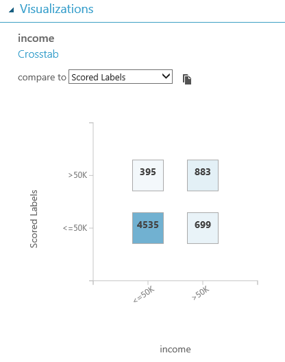
Now, let's take a look at the Contingency Table from the Cross-Validate Model tool, and compare it to the tables from the other posts.
 |
| Contingency Table (Two-Class Averaged Perceptron) |
 |
| Contingency Table (Two-Class Boosted Decision Tree) |
 |
| Contingency Table (Two-Class Logistic Regression) |
As you can see, all three of the algorithms are close when it comes to correctly predicting "<=50k". The story changes when it comes to ">50k". While the Two-Class Logistic Regression algorithm is better than the Two-Class Averaged Perceptron algorithm, it isn't quite as good as the Two-Class Boosted Decision Tree. We should point out that comparing these contingency tables is only a small part of choosing the "best" model. We can go more in-depth on model selection in a later post. Thanks for reading. We hope you found this informative.
Brad Llewellyn
BI Engineer
Valorem Consulting
@BreakingBI
www.linkedin.com/in/bradllewellyn
llewellyn.wb@gmail.com