Today, we're going to continue our walkthrough of the "Classifying_Iris" template provided as part of the AML Workbench. Previously, we've looked at
Getting Started and
Utilizing Different Environments. In this post, we're going to focus on the built-in data source options that the AML Workbench provides.
 |
| Data |
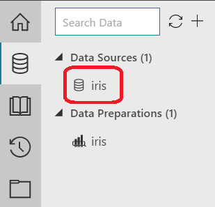
Let's start by opening the Data pane from the left side of the window.
 |
| Data Pane |
Here, we have the option of selecting "Data Sources" or "Data Preparations". "Data Sources" are what we use to bring our data in, as well perform some basic transformations to our data. "Data Transformations" give us quite a few more options for transform and clean our data. Additionally, we can have multiple "Data Transformations" using the same "Data Source". This allows us to create separate datasets for testing different types of transformations or for creating different datasets entirely using the same base dataset. Let's take a look at the "Data Source"
 |
| iris Data Source |
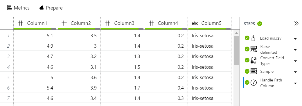
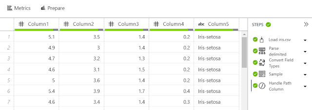
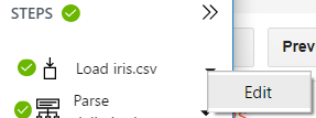
In this tab, we can see a few different areas. First, we can see the result of our data import in tabular format. This gives us a quick glance at what the data looks like. On the right side of the screen, we can see the steps that were taken to generate this data source. For those familiar with the Query Editor in Power BI (formerly known as Power Query), this is a very similar interface. We can alter any of the steps by clicking on the arrow beside them and selecting "Edit". Let's do this for the first step, "Load iris.csv".
 |
| Edit Data Source |
 |
| Edit Data Source Path |
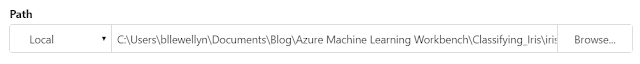
In this situation, the only option is to edit the location of the Data Source. You can read more about supported data formats
here.
Despite its spreadsheet feel and list of applied steps, the "Data Source" section has very few options. In fact, the steps we see utilized are ALL of the steps available. We cannot do any data transformation or manipulation in this tab. However, we do have an interesting option at the top of the tab called "Metrics".
 |
| Metrics |
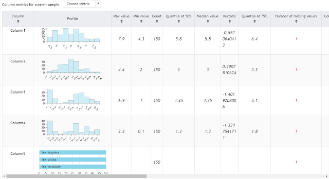 |
| iris Metrics |
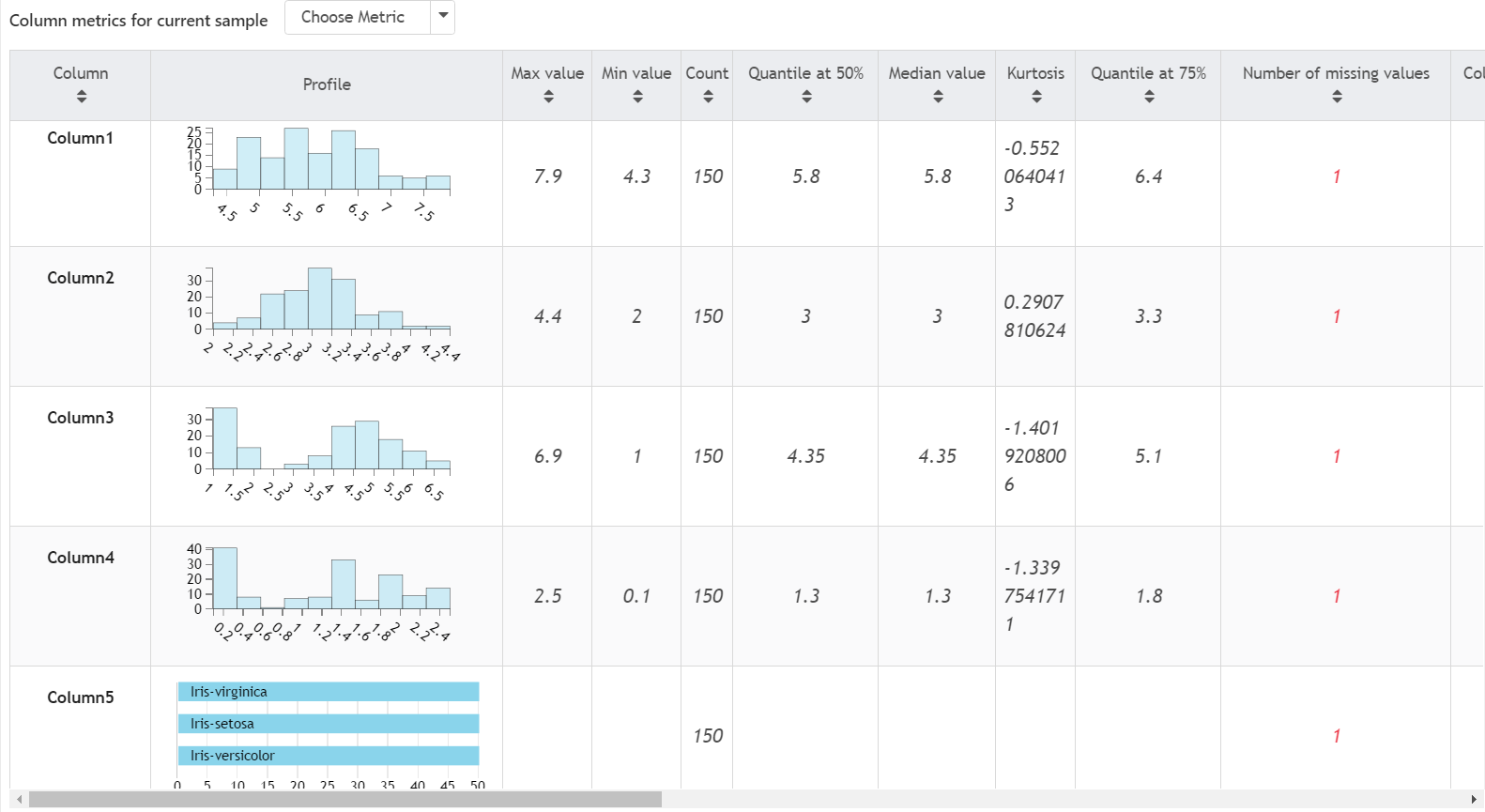
In this view, we can see a quick profile of the data (either a histogram or a bar chart based on the type of column), as well as a long list of metrics. Here's a summary of the metrics provided.
Max Value: Largest Value in the Column
Min Value: Smallest Value in the Column
Count: Number of Records with Values in this column
Quantile at 50%: A measure of the "central" value in a dataset. If the dataset was sorted, 50% of the values would be equal to or below this value.
Median: Same as Quantile at 50%
Kurtosis: Steepness of the distribution, i.e. a measure of the number of extreme observations it generates.
Quantile at 75%: If the dataset was sorted, 75% of the values would be equal to or below this value.
Number of Missing Values: Number of Records with No Value in this column
Column Data Type: The type of values that appears in the column.
Standard Deviation: Spread of the distribution, i.e. a measure of the distance between values in the column.
Variance: Spread of the distribution, i.e. a measure of the distance between values in the column., i.e. a measure of the distance between values in the column. This is the square of the Standard Deviation.
Quantile at 25%: If the dataset was sorted, 25% of the values would be equal to or below this value.
Is Numeric Column: Whether the values in the columns are numbers and have the appropriate data type to match.
Number of NaNs: The number of records that contain values which are not numbers. This does not consider the data type of the column and does not include missing values.
Mean Value: A measure of the "central" value in a dataset. Calculated as the sum of all values in the column, divided by the number of values. Commonly referred to as the "Average".
Unbiased Standard Error of the Mean: A measure of the stability of "Sample Mean" across samples. If we assume our dataset is a sample of a larger distribution, then that distribution likely has a Mean. However, since our sample is only part of the overall distribution, the mean of the sample will take different values based on which records are included in the sample. Therefore, we can say that the sample mean has it's own distribution, known as a "Sampling Distribution". This distribution likely has a standard deviation. This is known as the "standard error of the sample mean".
Skewness: A measure of how
NOT symmetric the distribution is, i.e. positive values signify the data has outliers larger than the mean, negative values signify the data has outliers smaller than the mean.
Most Common: The most common value in the column. Commonly called the "Mode". This only
applies to non-numeric columns.
Count of Most Common: The number of Records that contain the most common value. This only applies to non-numeric columns.
Number of Unique Values: The number of distinct values within the column, i.e. every distinct value is counted only once, regardless of how many times it appears in the column.
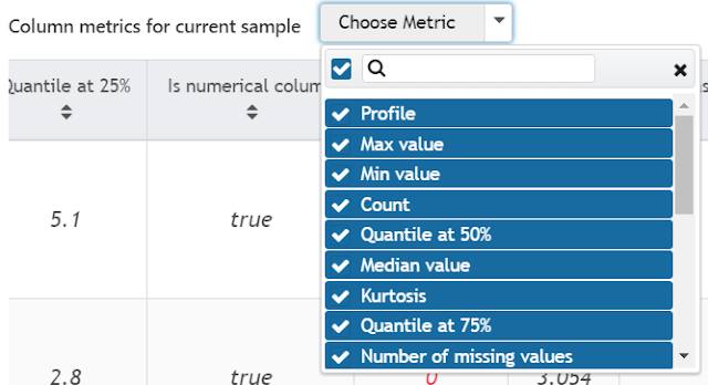 |
| Metrics Filter |
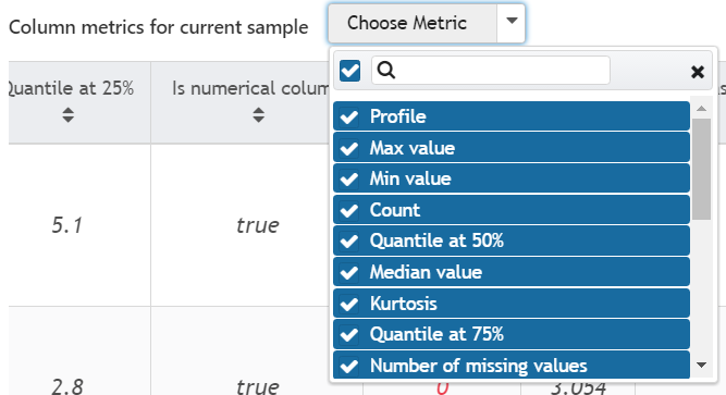
At the top of Metrics view, we also have the ability to filter the metrics we see. This is a great way to get a view of only the information we are interested in.
 |
| Prepare (from Data view) |
 |
| Prepare (from Metrics view) |
At the top of the Data Source tab, regardless of whether we are looking at the Data or Metrics view, there's another option called "Prepare". This will take us to the Data Preparations tab, which functions very similarly to the Query Editor in Power BI. We'll cover this in the next post.
Instead of going through the rest of the options available for editing in the Data Sources tab, let's create a new data source to see it from scratch. We've made a copy of the "iris.csv" file on our local machine.
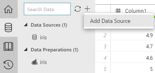 |
| Add Data Source |
At the top of the Data pane, we can click on the "+" button, then "Add Data Source".
 |
| Data Store |
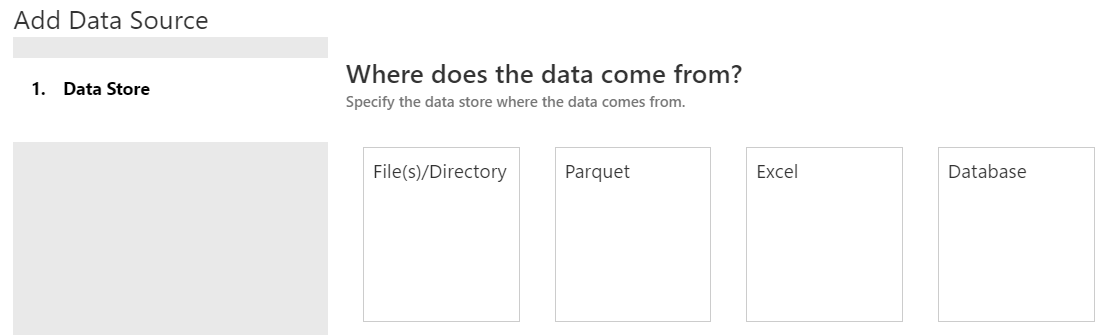
On the next screen, we have the option of choosing where our data comes from. We have a few different options. We can read files from our local machine or blob storage. We can read Parquet files from our local machine. Parquet is an open-source columnar file format common with big data solutions. You can read more about it
here. We can also read from Excel files in local or blob storage. Finally, we can read from a SQL Server Database as well. For more information on Data Sources, read
this. In our case, we want to pull from a csv on our local machine. Therefore, we want to use the File(s)/Directory option.
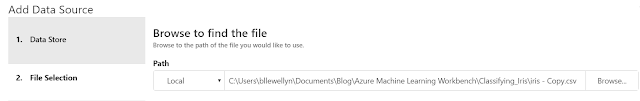 |
| File Selection |
In the next tab, we select the file(s) that we want to import. In our case, this is the "iris - Copy.csv" file from our local machine.
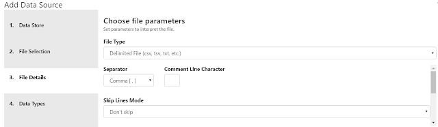 |
| File Details 1 |
 |
| File Details 2 |
 |
| File Details 3 |
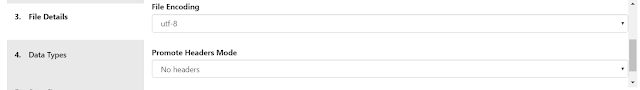
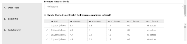
The next tab, "File Details" has some awkward scrolling. So, we had to make some interesting screenshot decisions to capture everything. On this tab, AML Workbench has already looked at the file and guessed at most of these properties. However, if we want to, we can change them. We get to define our File Type. The options are "Delimited File", "Fixed-Width File", "Plain Text File" and "JSON File". In our case, we want to use a "Delimited File" with a Separator of "Comma". We also get to decide whether we want to skip the first few lines. In our case we do not want to do this. We can also choose our File Encoding. There are a number of options here. In our case, we want to use utf-8. We can also let the tool know whether our file(s) have headers, i.e. column names. In this case, we do not. The last option is whether we want to handle Quoted Line Breaks. Honestly, we have no idea what this means as we've never seen it before. Perhaps someone in the comments can let us know. Finally, we get to see the results of our selections at the bottom of the tab.
 |
| Data Types 1 |
 |
| Data Types 2 |
On the next tab, AML Workbench automatically detects data types. However, it's always a good idea to check them in case we have to make some changes. The built-in options are "Numeric", "Date", "Boolean" (TRUE/FALSE) and "String". These options all look correct. It's also important to notice that AML Workbench added a field to the front of our dataset called "Path". Since we only used one file, this field is pretty worthless. However, if we were to pull in files from a directory, this could be a great to determine which file a record came from.
 |
| Sampling |
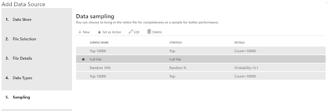
Depending on the size of the file, we may want to work with a sample to improve performance. The available options are "Top N", "Full File", "Random N%" and "Random N", with a default of "Top 10,000". Our file is small; so there's no harm in pulling in the full file. As we see above, we can also create multiple sampling rules, then choose which one we want to be active. This is an easy way to develop using a sample, then swap over to "Full File" when we're ready for full-scale testing. Depending on your Python skills, you may also consider utilizing more complex sampling techniques later using a Python notebook. We'll cover these in a later post.
 |
| Path Column |
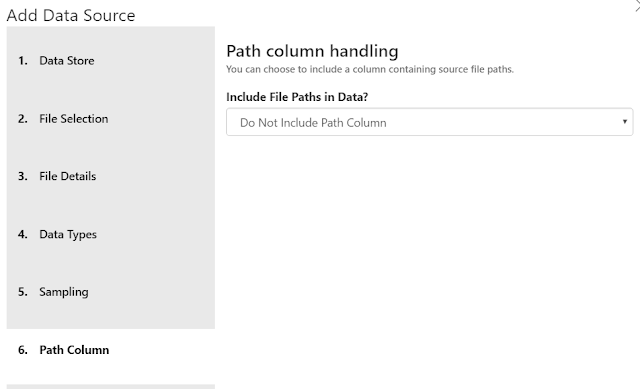
Finally, we get to choose whether we want to include the path column in our output data. As we talked about earlier, there's no reason to include it in this case.
 |
| iris - Copy Data Source |
Hopefully this post opened your eyes to the different possibilities for importing data into Azure Machine Learning Workbench. This is an extremely powerful tool and we've only begun to scratch the surface. Stay tuned for the next post where we'll walk through the Built-In Data Preparations. Thanks for reading. We hope you found this informative.
Brad Llewellyn
Senior Analytics Associate - Data Science
Syntelli Solutions
@BreakingBI
www.linkedin.com/in/bradllewellyn
llewellyn.wb@gmail.com