We haven't covered Power Query in a very long time on this blog. Since our last post in 2013, it's been fully integrated into the Power BI Desktop tool. Power Query is now known as the Power BI Query Editor and is a fully-functional ETL (Extract, Transform, Load) tool capable of pulling data from many data sources and integrating them into a single Power BI Data Model. You can read more about it here.
The first step is to load some data using the "Get Data" feature in Power BI.
 |
| Get Data |
 |
| Connect to Azure SQL Database |
 |
| SQL Server Database |
 |
| Navigator |
In the "Navigator" window, we want to select the Customer, Product, SalesOrderDetail and SalesOrderHeader tables. Now, we can use "Edit Queries" to access the Query Editor.
 |
| Edit Queries |
 |
| Power Query Editor |
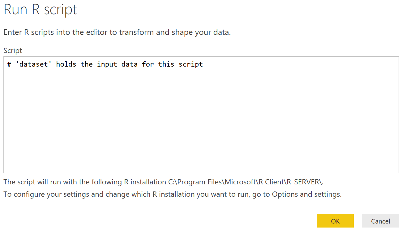
Once in the Query Editor, we can see the queries that pull in our four tables, as well as previews of these tables. The Query Editor has a tremendous amount of built-in capabilities to do any type of traditional data transformations. We're interested in the R functionality. Starting from the SalesLT SalesOrderHeader table, in the "Transform" tab, we can select "Run R Script" to open a scripting window.
 |
| Run R Script |
 |
| R Script Editor |
If you aren't able to open the R Script Editor, check out our previous post, Getting Started with R Scripts. While it's possible to develop and test code using the built-in R Script Editor, it's not great. Unfortunately, there doesn't seem to be a way to develop this script using an external IDE like RStudio. So, we typically export files to csv for development in RStudio. This is obviously not optimal and should be done with caution when data is extremely large or sensitive in some way. Fortunately, the write.csv() function is pretty easy to use. You can read more about it here.
<CODE START>
write.csv( dataset, file = <path> )
<CODE END>
<CODE START>
write.csv( dataset, file = <path> )
<CODE END>
 |
| Write to CSV |
 |
| Read from CSV |
Looking at this dataset, we see that it contains a number of fields. The issue is that it seems to contains a bunch of strange text values such as "Microsoft.OleDb.Currency", "[Value]" and "[Table]". These are caused by Base R not being able to interpret these Power Query datatypes. Obviously, there's nothing we can do with these fields in this format. So, we'll use Power Query to trim the dataset to only the columns we want and change the datatype of all of the other columns to numeric or text. To avoid delving too deep into Base Power Query, here's the M code to accomplish this. M is the language that the Query Editor automatically generates for you.
<CODE START>
#"Removed Columns" = Table.RemoveColumns(SalesLT_SalesOrderHeader,{"SalesLT.Address(BillToAddressID)", "SalesLT.Address(ShipToAddressID)", "SalesLT.Customer", "SalesLT.SalesOrderDetail"}),
#"Changed Type" = Table.TransformColumnTypes(#"Removed Columns",{{"TotalDue", type number}, {"Freight", type number}, {"TaxAmt", type number}, {"SubTotal", type number}}),
<CODE END>
 |
| Clean Data |
Looking at the new data, we can see that it's now clean enough to work with in R. Next, we'll do some basic R transformations to get a hang of it. Let's start by removing all columns from the data frame except for SalesOrderID, TaxAmt and TotalDue. We'll post the code later in the post.
 |
| Tax |
Now, let's create a new column "TaxPerc" that is calculated as "TaxAmt" / "TotalDue".

We can see that the tax percentages all hover right around 7.2%. It looks like the difference is probably just rounding error. Nevertheless, let's see how this outputs to the Query Editor.
 |
| Tax in Query Editor |
We can see the same data in Power Query that we saw in RStudio. This leads to the question "How did Power Query know to use the tax data frame as the next step?" If we look at the "Applied Steps" pane on the right side of the screen, we see that the Query Editor added a "tax" step without asking us. If we select the "Run R Script" step, we can see what the intermediate results looked like.
 |
| Run R Script in Query Editor |
Apparently, the Query Editor pulls back every data frame that was created in the R script. In this case, there was only one, so it expanded it automatically. We can confirm this by altering the R code to create a new data frame that similarly calculates "FreightPerc".
 |
| Tax and Freight in Query Editor |
Here's the code we used to generate this.
<CODE START>
tax <- dataset[,c("SalesOrderID", "TaxAmt", "TotalDue")]
tax[,"TaxPerc"] <- tax[,"TaxAmt"] / tax[,"TotalDue"]
freight <- dataset[,c("SalesOrderID", "Freight", "TotalDue")]
freight[,"FreightPerc"] <- freight[,"Freight"] / freight[,"TotalDue"]
<CODE END>
Obviously, we could use the fundamentals we just learned, combined with what we worked on in our previous post <INSERT LINK HERE> to build some predictive models here. Feel free to try that out on your own. For now, we'd rather look at some slightly different functionality.
There are a number of libraries that allow us to use R to perform data manipulation exercises, such as aggregations and joins. One of the more common packages is "dplyr". You can read more about it here. Let's install this package using RStudio and get started. If you need a refresher on how to install packages, check out this post.
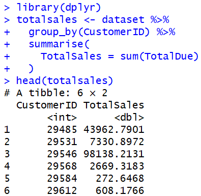
Now, let's start by calculating the total sales per customer.
 |
| Total Sales by Customer |
We see that the dplyr syntax is pretty simple and feels similar to SQL. However, these functions don't output data frames. Instead, they output tibbles. Fortunately, the Query Editor can read these with no issues.
 |
| Total Sales in Query Editor |
Here's the code we used.
<CODE START>
library(dplyr)
totalsales <- dataset %>%
group_by(CustomerID) %>%
summarise(
TotalSales = sum(TotalDue)
)
<CODE END>
Finally, let's take a look at table joins using dplyr. In order to do this, we need a way to bring two tables into the R script once. Fortunately, we can do this by tampering with the M code directly.
| Blank R Script |
If we look at our existing Power Query query, we see that the Query Editor leverages the R.Execute() function with an additional parameter at the end that says '[dataset=#"ChangedType"]'. This tells M to bring in the #"Changed Type" object into R and assign it to the dataset data frame. The #"Changed Type" object in the Query Editor is simply the temporary table created by our previous applied step.
 |
| Changed Type |
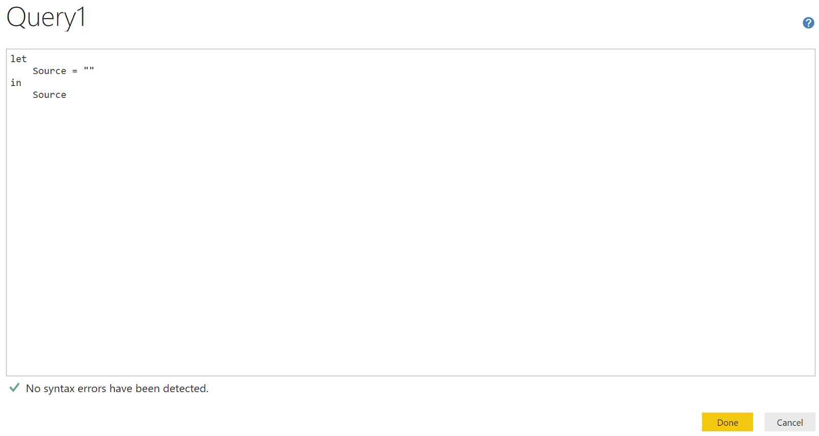
First, let's create a Blank M Script.
| Blank Query |
 |
| Advanced Editor |
 |
| Advanced Editor Window |
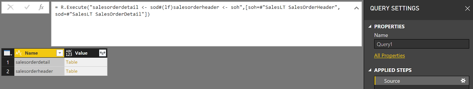
Here, we see an empty M query. Let's use the R.Execute() function to pull in two other queries in the Query Editor.
 |
| Two Tables |
Here's the code we used to generate this.
<M CODE START>
let
Source = R.Execute("salesorderdetail <- sod#(lf)salesorderheader <- soh",[soh=#"SalesLT SalesOrderHeader", sod=#"SalesLT SalesOrderDetail"])
in
Source
<M CODE END>
<R CODE START>
salesorderdetail <- sod
salesorderheader <- soh
<R CODE END>
We also dropped a few unnecessary columns from the SalesOrderDetail table and changed some data types to avoid the issues we saw earlier. Let's join these tables using the "SalesOrderID" key.
 |
| Joined in Query Editor |
Here's the code we used.
<CODE START>
library(dplyr)
joined <- inner_join(sod, soh, by = c("SalesOrderID"))
<CODE END>
We see that it's very easy to do this as well. In fact, it's possible to add joins to the "%>%" structure we were doing before. To learn more about these techniques, read this.
Hopefully, this post enlightened you as to some ways to add the power of R to your Power BI Queries. Not to give it all away, but we'll showcase some very interesting ways to build on these capabilities in the coming posts. Stay tuned for the next post where we'll take a look at the new Python functionality. Thanks for reading. We hope you found this informative.
Brad Llewellyn
Senior Analytics Associate - Data Science
Syntelli Solutions
@BreakingBI
www.linkedin.com/in/bradllewellyn
llewellyn.wb@gmail.com
Brad Llewellyn
Senior Analytics Associate - Data Science
Syntelli Solutions
@BreakingBI
www.linkedin.com/in/bradllewellyn
llewellyn.wb@gmail.com