So far in this experiment, we've taken the standard Azure Machine Learning evaluation metrics without much thought. However, an important thing to note is that all of these evaluation metrics assume that the prediction should be positive when the predicted is probability is greater than .5 (or 50%), and negative otherwise. This doesn't have to be the case.
In order to optimize the threshold for our data, we need a data set, a model and a module that optimizes the threshold for the data set and model. We already have a data set and a model, as we've spent the last few post building those. What we're missing is a module to optimize the threshold. For this, we're going to use an Execute R Script.
 |
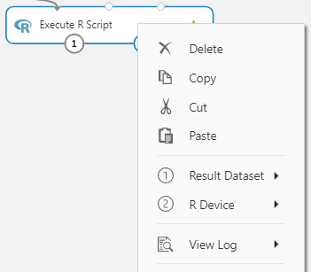
| Execute R Script |
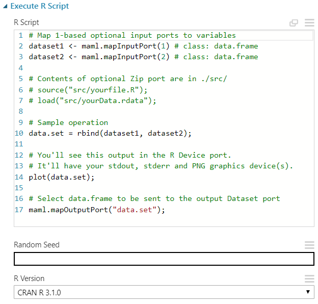 |
| Execute R Script Properties |
CODE BEGIN
dat <- maml.mapInputPort(1)
###############################################################
## Actual Values must be 0 for negative, 1 for positive.
## String Values are not allowed.
##
## You must supply the names of the Actual Value and Predicted
## Probability columns in the name.act and name.pred variables.
##
## In order to hone in on an optimal threshold, alter the
## values for min.out and max.out.
##
## If the script takes longer than a few minutes to run and the
## results are blank, reduce the num.thresh value.
###############################################################
name.act <- "Class"
name.pred <- "Scored Probabilities"
name.value <- c("Scored Probabilities")
num.thresh <- 1000
thresh.override <- c()
num.out <- 20
min.out <- -Inf
max.out <- Inf
num.obs <- length(dat[,1])
cost.tp.base <- 0
cost.tn.base <- 0
cost.fp.base <- 0
cost.fn.base <- 0
#############################################
## Choose an Optimize By option. Options are
## "totalcost", "precision", "recall" and
## "precisionxrecall".
#############################################
opt.by <- "precisionxrecall"
act <- dat[,name.act]
act[is.na(act)] <- 0
pred <- dat[,name.pred]
pred[is.na(pred)] <- 0
value <- -dat[,name.value]
value[is.na(value)] <- 0
#########################
## Thresholds are Defined
#########################
if( length(thresh.override) > 0 ){
thresh <- thresh.override
num.thresh <- length(thresh)
}else if( num.obs <= num.thresh ){
thresh <- sort(pred)
num.thresh <- length(thresh)
}else{
thresh <- sort(pred)[floor(1:num.thresh * num.obs / num.thresh)]
}
#######################################
## Precision/Recall Curve is Calculated
#######################################
prec <- c()
rec <- c()
true.pos <- c()
true.neg <- c()
false.pos <- c()
false.neg <- c()
act.true <- sum(act)
cost.tp <- c()
cost.tn <- c()
cost.fp <- c()
cost.fn <- c()
cost <- c()
for(i in 1:num.thresh){
thresh.temp <- thresh[i]
pred.temp <- as.numeric(pred >= thresh.temp)
true.pos.temp <- act * pred.temp
true.pos[i] <- sum(true.pos.temp)
true.neg.temp <- (1-act) * (1-pred.temp)
true.neg[i] <- sum(true.neg.temp)
false.pos.temp <- (1-act) * pred.temp
false.pos[i] <- sum(false.pos.temp)
false.neg.temp <- act * (1-pred.temp)
false.neg[i] <- sum(false.neg.temp)
pred.true <- sum(pred.temp)
prec[i] <- true.pos[i] / pred.true
rec[i] <- true.pos[i] / act.true
cost.tp[i] <- cost.tp.base * true.pos[i]
cost.tn[i] <- cost.tn.base * true.neg[i]
cost.fp[i] <- cost.fp.base * false.pos[i]
cost.fn[i] <- cost.fn.base * false.neg[i]
}
cost <- cost.tp + cost.tn + cost.fp + cost.fn
prec.ord <- prec[order(rec)]
rec.ord <- rec[order(rec)]
plot(rec.ord, prec.ord, type = "l", main = "Precision/Recall Curve", xlab = "Recall", ylab = "Precision")
######################################################
## Area Under the Precision/Recall Curve is Calculated
######################################################
auc <- c()
for(i in 1:(num.thresh - 1)){
auc[i] <- prec.ord[i] * ( rec.ord[i + 1] - rec.ord[i] )
}
#################
## Data is Output
#################
thresh.out <- 1:num.thresh * as.numeric(thresh >= min.out) * as.numeric(thresh <= max.out)
num.thresh.out <- length(thresh.out[thresh.out > 0])
min.thresh.out <- min(thresh.out[thresh.out > 0])
if( opt.by == "totalcost" ){
opt.val <- cost
}else if( opt.by == "precision" ){
opt.val <- prec
}else if( opt.by == "recall" ){
opt.val <- rec
}else if( opt.by == "precisionxrecall" ){
opt.val <- prec * rec
}
ind.opt <- order(opt.val, decreasing = TRUE)[1]
ind.out <- min.thresh.out + floor(1:num.out * num.thresh.out / num.out) - 1
out <- data.frame(rev(thresh[ind.out]), rev(true.pos[ind.out]), rev(true.neg[ind.out]), rev(false.pos[ind.out]), rev(false.neg[ind.out]), rev(prec[ind.out]), rev(rec[ind.out]), rev(c(0, auc)[ind.out]), rev(cost.tp[ind.out]), rev(cost.tn[ind.out]), rev(cost.fp[ind.out]), rev(cost.fn[ind.out]), rev(cost[ind.out]), rev(c(0,cumsum(auc))[ind.out]), thresh[ind.opt], prec[ind.opt], rec[ind.opt], cost.tp[ind.opt], cost.tn[ind.opt], cost.fp[ind.opt], cost.fn[ind.opt], cost[ind.opt])
names(out) <- c("Threshold", "True Positives", "True Negatives", "False Positives", "False Negatives", "Precision", "Recall", "Area Under P/R Curve", "True Positive Cost", "True Negative Cost", "False Positive Cost", "False Negative Cost", "Total Cost", "Cumulative Area Under P/R Curve", "Optimal Threshold", "Optimal Precision", "Optimal Recall", "Optimal True Positive Cost", "Optimal True Negative Cost", "Optimal False Positive Cost", "Optimal False Negative Cost", "Optimal Cost")
maml.mapOutputPort("out");
###############################################################
## Actual Values must be 0 for negative, 1 for positive.
## String Values are not allowed.
##
## You must supply the names of the Actual Value and Predicted
## Probability columns in the name.act and name.pred variables.
##
## In order to hone in on an optimal threshold, alter the
## values for min.out and max.out.
##
## If the script takes longer than a few minutes to run and the
## results are blank, reduce the num.thresh value.
###############################################################
name.act <- "Class"
name.pred <- "Scored Probabilities"
name.value <- c("Scored Probabilities")
num.thresh <- 1000
thresh.override <- c()
num.out <- 20
min.out <- -Inf
max.out <- Inf
num.obs <- length(dat[,1])
cost.tp.base <- 0
cost.tn.base <- 0
cost.fp.base <- 0
cost.fn.base <- 0
#############################################
## Choose an Optimize By option. Options are
## "totalcost", "precision", "recall" and
## "precisionxrecall".
#############################################
opt.by <- "precisionxrecall"
act <- dat[,name.act]
act[is.na(act)] <- 0
pred <- dat[,name.pred]
pred[is.na(pred)] <- 0
value <- -dat[,name.value]
value[is.na(value)] <- 0
#########################
## Thresholds are Defined
#########################
if( length(thresh.override) > 0 ){
thresh <- thresh.override
num.thresh <- length(thresh)
}else if( num.obs <= num.thresh ){
thresh <- sort(pred)
num.thresh <- length(thresh)
}else{
thresh <- sort(pred)[floor(1:num.thresh * num.obs / num.thresh)]
}
#######################################
## Precision/Recall Curve is Calculated
#######################################
prec <- c()
rec <- c()
true.pos <- c()
true.neg <- c()
false.pos <- c()
false.neg <- c()
act.true <- sum(act)
cost.tp <- c()
cost.tn <- c()
cost.fp <- c()
cost.fn <- c()
cost <- c()
for(i in 1:num.thresh){
thresh.temp <- thresh[i]
pred.temp <- as.numeric(pred >= thresh.temp)
true.pos.temp <- act * pred.temp
true.pos[i] <- sum(true.pos.temp)
true.neg.temp <- (1-act) * (1-pred.temp)
true.neg[i] <- sum(true.neg.temp)
false.pos.temp <- (1-act) * pred.temp
false.pos[i] <- sum(false.pos.temp)
false.neg.temp <- act * (1-pred.temp)
false.neg[i] <- sum(false.neg.temp)
pred.true <- sum(pred.temp)
prec[i] <- true.pos[i] / pred.true
rec[i] <- true.pos[i] / act.true
cost.tp[i] <- cost.tp.base * true.pos[i]
cost.tn[i] <- cost.tn.base * true.neg[i]
cost.fp[i] <- cost.fp.base * false.pos[i]
cost.fn[i] <- cost.fn.base * false.neg[i]
}
cost <- cost.tp + cost.tn + cost.fp + cost.fn
prec.ord <- prec[order(rec)]
rec.ord <- rec[order(rec)]
plot(rec.ord, prec.ord, type = "l", main = "Precision/Recall Curve", xlab = "Recall", ylab = "Precision")
######################################################
## Area Under the Precision/Recall Curve is Calculated
######################################################
auc <- c()
for(i in 1:(num.thresh - 1)){
auc[i] <- prec.ord[i] * ( rec.ord[i + 1] - rec.ord[i] )
}
#################
## Data is Output
#################
thresh.out <- 1:num.thresh * as.numeric(thresh >= min.out) * as.numeric(thresh <= max.out)
num.thresh.out <- length(thresh.out[thresh.out > 0])
min.thresh.out <- min(thresh.out[thresh.out > 0])
if( opt.by == "totalcost" ){
opt.val <- cost
}else if( opt.by == "precision" ){
opt.val <- prec
}else if( opt.by == "recall" ){
opt.val <- rec
}else if( opt.by == "precisionxrecall" ){
opt.val <- prec * rec
}
ind.opt <- order(opt.val, decreasing = TRUE)[1]
ind.out <- min.thresh.out + floor(1:num.out * num.thresh.out / num.out) - 1
out <- data.frame(rev(thresh[ind.out]), rev(true.pos[ind.out]), rev(true.neg[ind.out]), rev(false.pos[ind.out]), rev(false.neg[ind.out]), rev(prec[ind.out]), rev(rec[ind.out]), rev(c(0, auc)[ind.out]), rev(cost.tp[ind.out]), rev(cost.tn[ind.out]), rev(cost.fp[ind.out]), rev(cost.fn[ind.out]), rev(cost[ind.out]), rev(c(0,cumsum(auc))[ind.out]), thresh[ind.opt], prec[ind.opt], rec[ind.opt], cost.tp[ind.opt], cost.tn[ind.opt], cost.fp[ind.opt], cost.fn[ind.opt], cost[ind.opt])
names(out) <- c("Threshold", "True Positives", "True Negatives", "False Positives", "False Negatives", "Precision", "Recall", "Area Under P/R Curve", "True Positive Cost", "True Negative Cost", "False Positive Cost", "False Negative Cost", "Total Cost", "Cumulative Area Under P/R Curve", "Optimal Threshold", "Optimal Precision", "Optimal Recall", "Optimal True Positive Cost", "Optimal True Negative Cost", "Optimal False Positive Cost", "Optimal False Negative Cost", "Optimal Cost")
maml.mapOutputPort("out");
CODE END
We created this piece of code to help us examine the area under the Precision/Recall curve (AUC in Azure Machine Learning Studio refers to the area under the ROC curve) and to determine the optimal threshold for our data set. It even allows us to input a custom cost function to determine how much money would have been saved and/or generated using the model. Let's take a look at the results.
 |
| Experiment |
 |
| Execute R Script Outputs |
 |
| Execute R Script Results 1 |
 |
| Execute R Script Results 2 |
 |
| Execute R Script Graphics |
#############################################
## Choose an Optimize By option. Options are
## "totalcost", "precision", "recall" and
## "precisionxrecall".
#############################################
opt.by <- "precisionxrecall"
In our case, we chose to optimize by using Precision * Recall. Looking back at the results from our "Execute R Script", we see that our thresholds jump all the way from .000591 to .983291. This is because the "Scored Probabilities" output from the "Score Model" module are very heavily skewed towards zero. In turn, this skew is caused by the fact that our "Class" variable is heavily imbalanced.
Because of the way the R code is built, it determined that the optimal threshold of .001316 has a Precision of 82.9% and a Recall of 90.6%. These values are worse than those originally reported by the "Tune Model Hyperparameters" module. So, we can override the thresholds in our R code using the following code at the top of the batch:
thresh.override <- (10:90)/100
This will tell the R script to forcibly use thresholds from .10 to .90. Let's check out the results.
We can see that by moving our threshold down to .42, we can tweak out slightly more value from our model. However, this is a such a small amount of value that it's not worth any amount of effort to do it in this case.
So, when would this be useful? As with everything, it all comes down to dollars. We can talk to stakeholders and clients all day about how much Accuracy, Precision and Recall our models have. In general, they aren't interested in that type of information. However, if we can input an estimate of their cost function into this script, then we can tie real dollars to the model. We were able to use this script to show a client that they could save $200k per year in lost product using their model. That had far more impact than a Precision value ever would.
Hopefully, this post sparked your interest in tuning your Azure Machine Learning models to maximize their effectiveness. We also want to emphasize that you can use R and Python to greatly extend the usefulness of Azure Machine Learning. Stay tuned for the next post where we'll be talking about Feature Selection. Thanks for reading. We hope you found this informative.
Brad Llewellyn
Data Scientist
Valorem
@BreakingBI
www.linkedin.com/in/bradllewellyn
llewellyn.wb@gmail.com
 |
| Scored Probabilities Statistics |
 |
| Scored Probabilities Histogram |
thresh.override <- (10:90)/100
This will tell the R script to forcibly use thresholds from .10 to .90. Let's check out the results.
 |
| Overridden Threshold Results 1 |
 |
| Overridden Threshold Results 2 |
So, when would this be useful? As with everything, it all comes down to dollars. We can talk to stakeholders and clients all day about how much Accuracy, Precision and Recall our models have. In general, they aren't interested in that type of information. However, if we can input an estimate of their cost function into this script, then we can tie real dollars to the model. We were able to use this script to show a client that they could save $200k per year in lost product using their model. That had far more impact than a Precision value ever would.
Hopefully, this post sparked your interest in tuning your Azure Machine Learning models to maximize their effectiveness. We also want to emphasize that you can use R and Python to greatly extend the usefulness of Azure Machine Learning. Stay tuned for the next post where we'll be talking about Feature Selection. Thanks for reading. We hope you found this informative.
Brad Llewellyn
Data Scientist
Valorem
@BreakingBI
www.linkedin.com/in/bradllewellyn
llewellyn.wb@gmail.com