Data Mining in Excel Part 25: Naive Bayes

Today, we're going to talk another of the "hidden" algorithms in the Data Mining Add-ins for Excel, Naive Bayes.  Naive Bayes is a classification algorithm, similar to Decision Trees and Logistic Regression, that attempts to predict categorical values.  A special catch of this procedure is that it can only use discrete and discretized values, meaning continuous values like Age and Income cannot be used.  If you want to use these types of values, then you would need to discretize them first.  To read more about Naive Bayes, navigate here.  In order to use this algorithm, we need to add another model to our existing structures using the "Add Model to Structure" button.

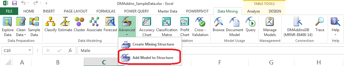Add Model to Structure

Let's get started.

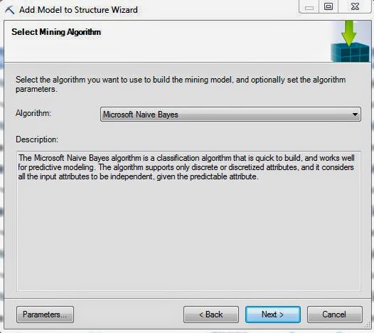Select Algorithm

First, we need to select the Naive Bayes algorithm.  Before we move on, let's take a look at the Parameters.

Parameters

Just like that with Logistic Regression, this algorithm have very few parameters.  In fact, the only parameter that actually affects the model is the Minimum Dependency Probability.  Altering this value will increase or decrease the number of predictors in the model.  For more information on these parameters, read this.  Let's move on.

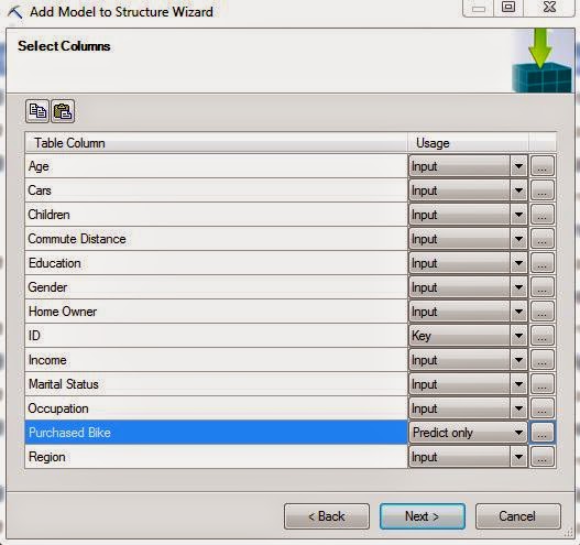
Select Columns

Since the structure has defined Age and Income as Continuous variables, this algorithm will not let us use them.  So, the only thing we need to change here is set Purchased Bike to "Predict Only".

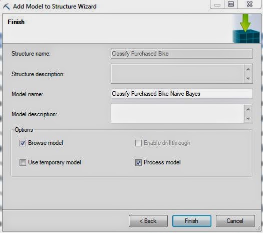Create Model

Finally, we create our model using the naming convention we've been following for this entire series.  It's important to note that, just like Logistic Regression, this algorithm doesn't support drillthrough.  Let's jump to the output.

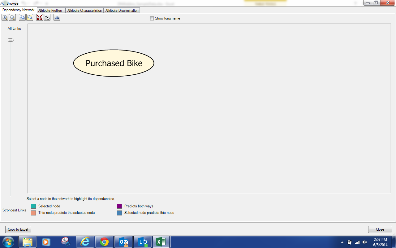Dependency Network

Well, we have an issue already.  There are no variables in the model other than Purchased Bike.  This means that we can't predict values with this model.  This is very likely due to the fact that the best predictors are discretized versions of Income and Age.  To test this, let's create another structure that discretizes those values and use that for a new model.  For more information on how to create a mining structure, read this.

Select Columns (Discretized)

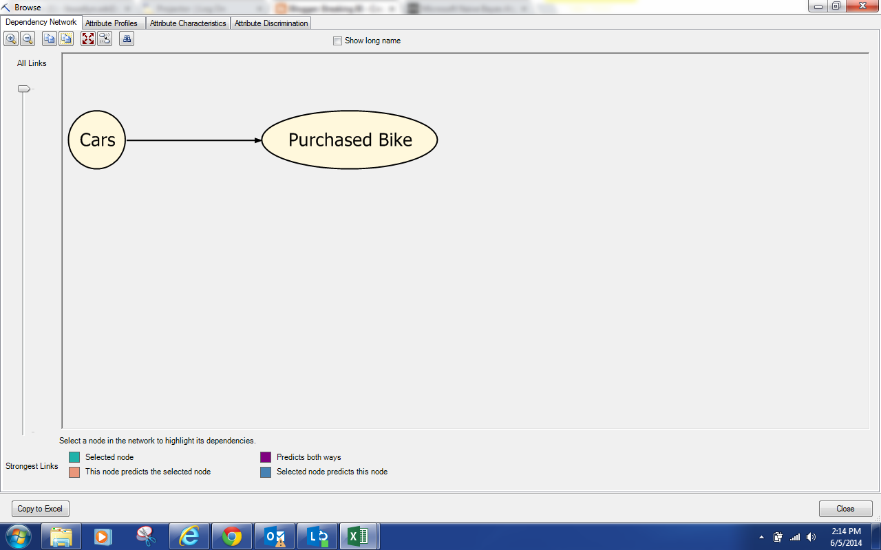
Notice how Age and Income are inputs now?  That's because they're no longer Continuous variables.  Let's check out this model.

Dependency Network (Discretized)

For some reason, discretizing Age and Income cause Cars to become statistically significant.  This model is still pretty bare, let's change the parameters to get a fuller model.

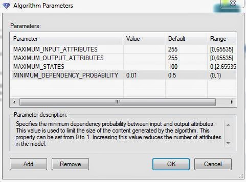
Parameters (.01 MDP)

We needed to reduce the Minimum Dependency Probability all the way to .01, which is almost as low as it can be, before we actually got any change in the model.  At this point, we're thoroughly convinced that this algorithm is not appropriate for this data set.  However, we'll continue the analysis as a demonstration.  Let's check out the model.

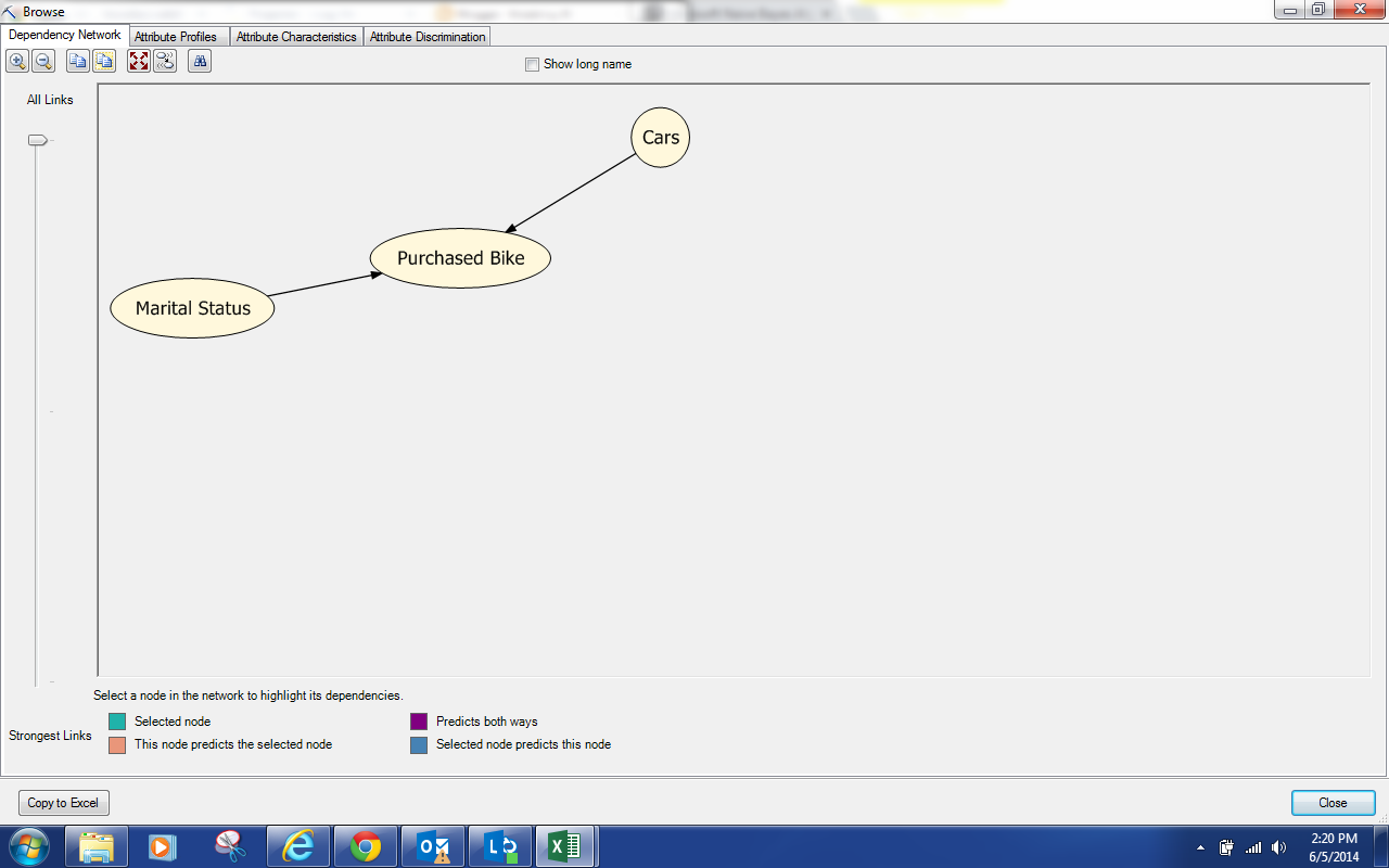
Dependency Network  (.01 MDP)

We see that Marital Status and Cars are predictors for Purchased Bike.  Next, let's jump over to Attribute Profiles.

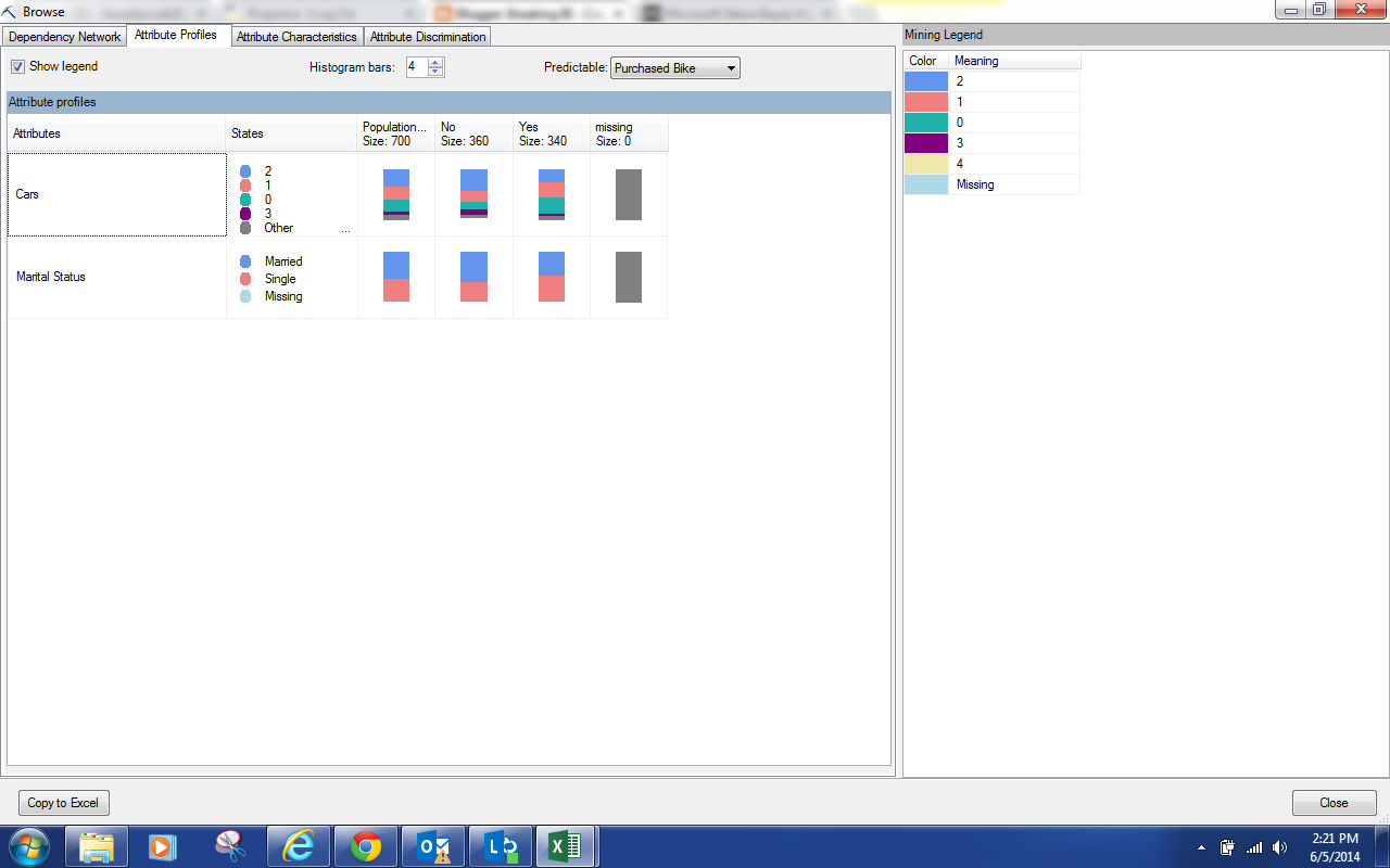Attribute Profiles

We can see the breakdown of each predictor as it relates to each value of Purchased Bike.  The differences are pretty minor.  So, let's move on to the Attribute Characteristics.

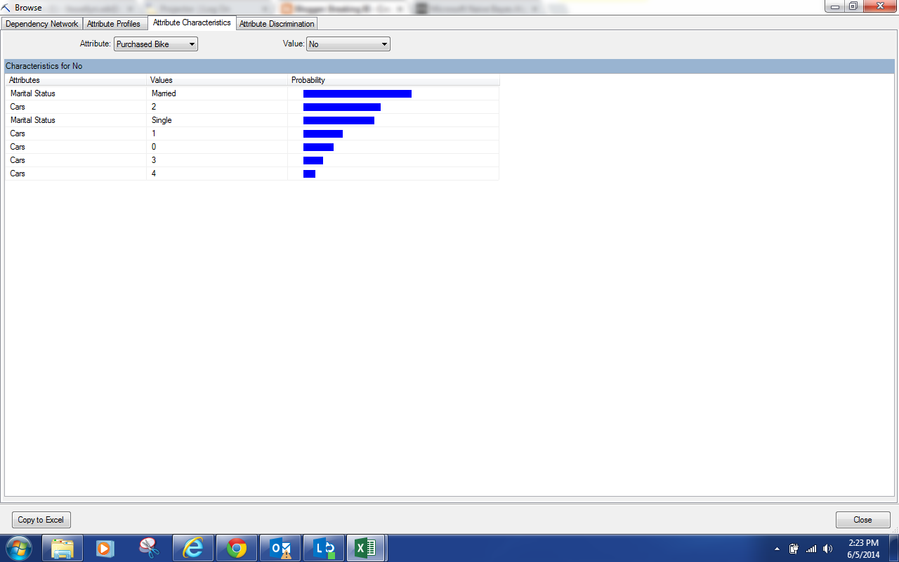Attribute Characteristics

By now, you should have noticed that this is exactly the same type of output we saw for the Clustering Algorithm, albeit less useful because of the quality of the model.  This screen shows us what makes up each individual value of Purchased Bike.  However, we find the Attribute Discrimination to be much more useful.

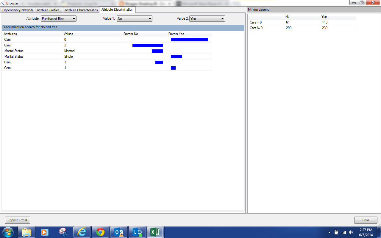Attribute Discrimination

This view will show you what attributes correspond best with certain outcomes.  Not surprisingly, we see that people with no cars tend to buy bikes while people with 2 cars do not.  We also see that married people don't usually buy bikes while Single people do.

Just like with Logistic Regression, this algorithm is typically not as useful as Decision Trees.  However, it will typically perform better.  So, the goal is to see whether the increase processing and querying time for the more complex models actually yields better predictions.  In this case, the Decision Tree model is significantly better.  Keep an eye for the next post where we'll be talking about Neural Networks.  Thanks for reading.  We hope you found this informative.

Brad Llewellyn
Director, Consumer Sciences
Consumer Orbit
llewellyn.wb@gmail.com

http://www.linkedin.com/in/bradllewellyn