Today, we will begin the next series of posts about performing predictive analysis via Tableau 8.1's new R functionality. More specifically, we'll be talking about Simple Linear Regression. Some of you may remember our previous post on this topic,
Performing Simple Linear Regression in Tableau. That procedure utilized Table Calculations, which despite being powerful in their own right, were not quite meant for such complex mathematics. The new R integration makes this task significantly easier, as we are about to see. For this procedure, we will use a sample data set from
a collegiate source.
The first question you might ask is "Why is this important?" Well, regression is one of the many ways in which you can predict new observations. Want to know what your sales will be next month for a particular product line? Regression can help. Want to know how many new customers you will acquire in the next 3 months? Regression can help. The list goes on and on. Now, all we need is a good foundation. Then, addressing many of your business problems would be within our grasp.
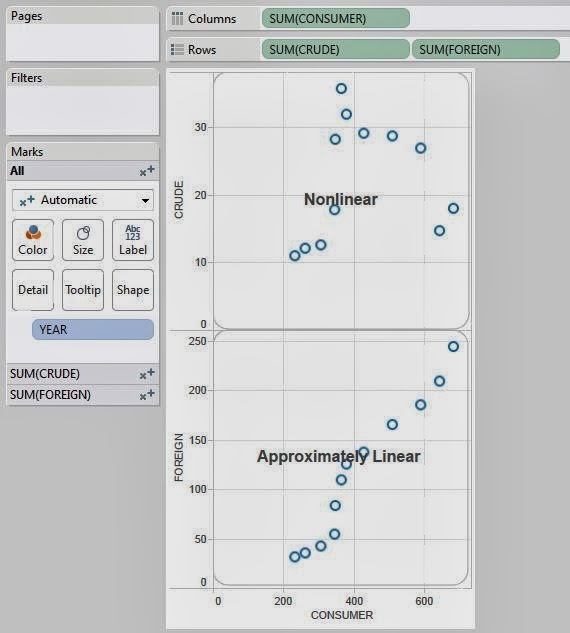
The first step of any regression model is determining which variables are going to be your predictors and which variables are going to be your responses. In a simple linear regression model, we can only have one predictor and one response. We also assume that they are related in a "linear" fashion, which is easiest understand via a picture.
 |
| Linear vs. Nonlinear |
Now, we can see that the relationship between Foreign and Consumer is approximately linear. However, some of you might ask, "What are these values?" These are U.S. Economic figures for the years between 1976 and 1987. Foreign is "Foreign Investments / Billions of Dollars" and Consumer is "Consumer Debt / Billions of Dollars." Now, let's try to predict how much we will have in foreign investments given that we know what consumer debt will be.
.JPG) |
| Foreign (Predicted) |
The code for creating a linear regression model is extremely simple, nothing more than two lines of actual code. Now, let's see what values we get.
 |
| Consumer, Foreign, and Predicted Foreign by Year |
Voila! We have predictions. However, it's difficult to see the relationship in a text table. Let's create a % Difference calculation and make this into a highlight table.
.JPG) |
| Consumer vs. Foreign (Highlight Table) |
Now we can easily see which predictions were close, and which were not so close. This was a bit too easy though, let's try something else. When you use a regression model to predict a value, you don't just get a single value, you actually get a range that the value is likely to be in. This is called a prediction interval. If you want a more rigorous definition, you can check out
this article. Now, what if we were to use R to calculate these intervals? Let's see!
.JPG) |
| Foreign (Predicted Lower) |
.JPG) |
| Foreign (Predicted Upper) |
These calculations leverage a neat function called predict() that we won't go into detail on at this time. However, it's one of R's many multi-purpose functions. Now, we just need a way to look at these. A little imagination goes a long way in these types of charts.
.JPG) |
| Consumer vs. Foreign (Banded Scatterplot) |
As you can see, all of our values fall within the bounds. This is a good thing. It means that our model fit our data pretty well.
The really cool part about this new R integration is definitely in the prediction and forecasting scenarios. As we just saw, it's really easy to get some cool predictions and display them. There's WAY more to do here. We could have gotten more technical by looking at residual plots or QQ plots. Don't think that linear regression was the right model? No problem! We could have used a time series, artificial neural network, or even a Bayesian model. You're only limited by your imagination. We hope you found this informative. Thanks for reading.
Data Analytics Consultant
Mariner, LLC
brad.llewellyn@mariner-usa.com
http://www.linkedin.com/in/bradllewellyn
http://breaking-bi.blogspot.com
.JPG)

.JPG)
.JPG)
.JPG)
.JPG)
Hi Brad,
ReplyDeleteGreat post around regression modelling. I just have a small questions. can we see the beta coefficients of all independent variables with dependent variable
Regards,
Ankit
Ankit,
DeleteOf course! This is just R code so you can do anything you want. I think the function for returning the coefficients is fit$coeff. However, the coefficients are at the same granularity as the data. So, you'll have to get a little more clever about displaying them. Basically, the R integration is great for predicting values, but pretty clunky when it comes to testing the model because the functions can only return the same number of observations as you give them
Hello Brad,
ReplyDeleteI have a requirement using R an tableau, The details are as follows,
can we pass the arguments(.arg1,arg2....) as parameters, so that user can select the X and Y variables in tableau using the parameter control and the visualization changes accordingly.?
Lets consider a Simple linear regression R script in tableau:
SCRIPT_int('
mydata <- data.frame(rooms <- .arg1, ok <-.arg2, af <- .arg3, rating <- .arg4, initial<-.arg5, time <- .arg6 );
lrmodel <- lm(time ~ as.factor(ok) + rooms + as.factor(af) + rating, data = mydata);
lrmodel$fitted
prob <- predict(lrmodel, newdata = mydata, type = "response")
',
ATTR([Number of Rooms]),
ATTR([OK or SUI]),
ATTR([AF Counted]),
ATTR([Rating]),
ATTR([Initial or Makeup]),
ATTR([total TIME])
)
Now the requirement is instead passing the variables directly for X and Y as arguments , pass the arguments as parameters??
Kindly let me know if this question makes sense, or if more information is needed?. Thanks awaiting for the reply.
Thanks and Regards
Yashwanth
Yashwanth,
DeleteJust create a calculated field that equals your parameter (ex. parameter "consumer spend", calculated field "consumer spend variable"). Initially, load the parameter with values from your field. The parameter won't have a dynamic range, but it will suffice for your needs. If you need to have the parameter be dynamic, there are ways to make it so.
how to get the percent of difference and how to calculate it?
ReplyDeleteHi Brad,
ReplyDeleteI'm using a similar formula and getting a strange error that I can't seem to sort out:
Unexpected number of results returned by SCRIPT function. Function expected 5206 values; 2268 values returned
Any thoughts on how to fix this? Here's my code
SCRIPT_REAL("
fit <- lm(.arg1 ~ .arg2 + .arg3)
fit$fitted
"
,
SUM([Applications (2015)]),
SUM([Applications (2014)]),
SUM([Applications (2013)])
)
How can we run the new data to predict the dependent variable basis on already established predictive model?
ReplyDeleteI am not able to run the lm function in the code. Do I need to install any package related to it in R first?
ReplyDeleteHi Brad, nice post, congratulation.
ReplyDeletewitch sample data set from a collegiate source did you pick? Please
What are the technical features available in Predictive analysis of BI????
ReplyDeleteHi is there a way that we can save the fit method some where (more precisely in Rserve session)and use the predict method for the calculated field ?
ReplyDelete