Before we install the AML Workbench, let's talk about what it is. The AML Workbench is a local environment for developing data science solutions that can be easily deployed and managed using Microsoft Azure. It doesn't appear to be related to AML Studio in any way. Throughout this series, we'll walk through all of the different things we can do with the AML Workbench. For today, we're just going to get our feet wet.
Now, we need to create an Azure Machine Learning Experimentation resource in the Azure portal. You can find complete instructions here. We will also include a Workspace and a Model Management Account. This appears to be free for the first two users. However, we're not sure whether they charge separately for the storage account. Maybe someone can let us know in the comments. Now, let's boot this baby up!
 |
| Azure Machine Learning Workbench |
 |
| New Project |
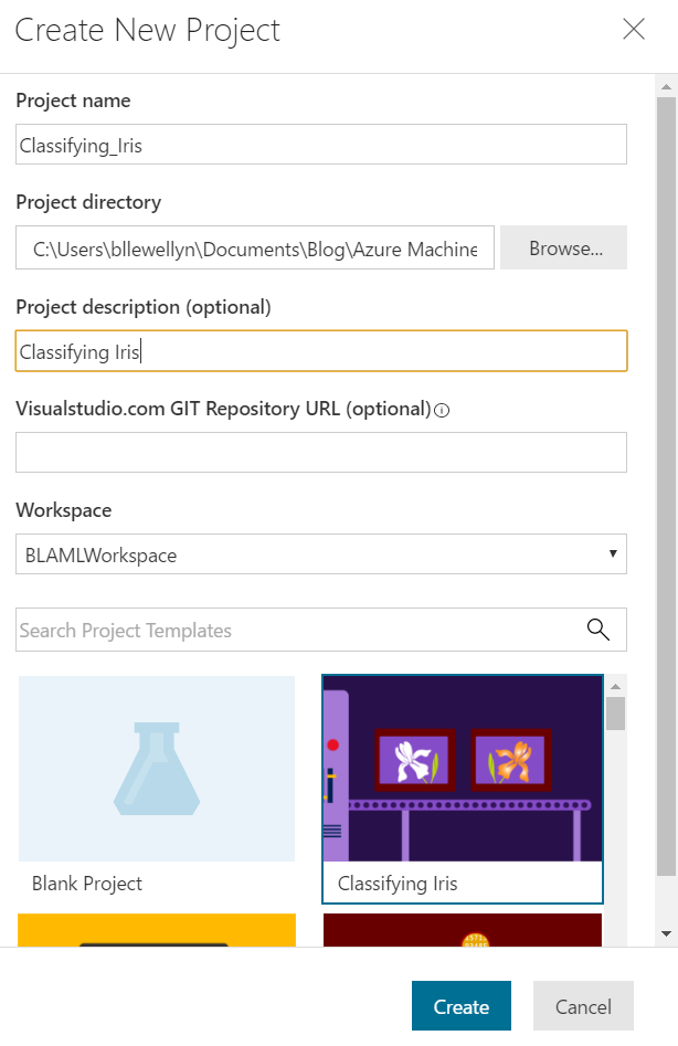 |
| Create New Project |
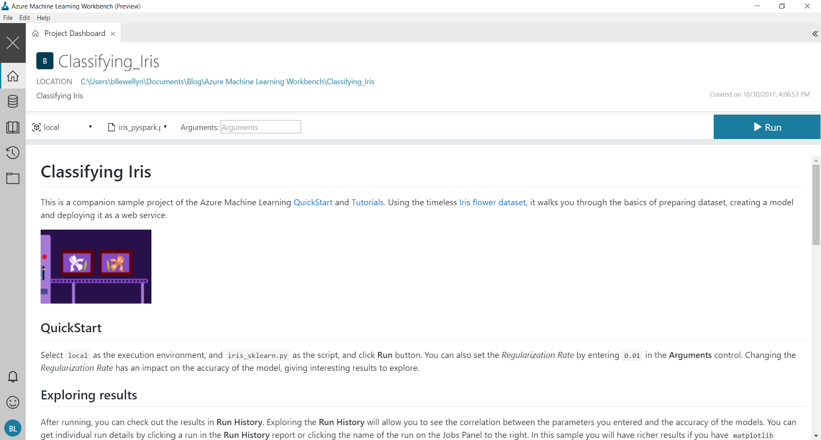 |
| Project Dashboard |
 |
| iris_sklearn |
 |
| Run History |
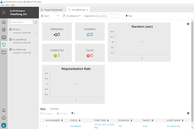 |
| iris_sklearn Run History |
 |
| Job History |
If we click on the Job Name in the Jobs section on the right side of the screen, we can see a more detailed result set.
 |
| Run Properties |
This is what we were looking for! This gives us all kinds of information about the run. This could be extremely useful for showing the results of an experiment to bosses or colleagues.
 |
| Logs |
Further down the page, we see the Logs section. This is where we can access all the granular information we would need if we needed to debug a particular issue.
The next section of the instructions is the Quick CLI Reference. This gives us a bunch of code we can use to run these scripts from the Command Line (or Powershell). Let's open a new command line window.
In the top-left corner of the window, we can select "Open Command Prompt" from the "File" menu.
In the command prompt, we can copy the first line of code from the instructions.
The next section of the instructions is the Quick CLI Reference. This gives us a bunch of code we can use to run these scripts from the Command Line (or Powershell). Let's open a new command line window.
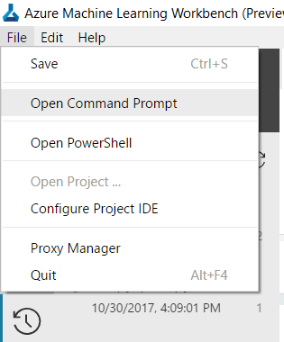 |
| Open Command Prompt |
 |
| Command Prompt |
pip install matplotlib
This code will install the Python library "matplotlib". This library contains quite a few functions for creating graphs in Python. You can read more about it here. Now that we have the library installed, let's copy the next line of code.
az login
This code will help us log the Command Line Interface into Azure. When we run this command, we get the following response.
The next piece of code we need to run is as follows.
OUTPUT BEGIN
RunId: Classifying_Iris_1509457170414
Executing user inputs .....
===========================
Python version: 3.5.2 |Continuum Analytics, Inc.| (default, Jul 5 2016, 11:41:13) [MSC v.1900 64 bit (AMD64)]
Iris dataset shape: (150, 5)
Regularization rate is 10.0
LogisticRegression(C=0.1, class_weight=None, dual=False, fit_intercept=True,
intercept_scaling=1, max_iter=100, multi_class='ovr', n_jobs=1,
penalty='l2', random_state=None, solver='liblinear', tol=0.0001,
verbose=0, warm_start=False)
Accuracy is 0.6415094339622641
==========================================
Serialize and deserialize using the outputs folder.
Export the model to model.pkl
Import the model from model.pkl
New sample: [[3.0, 3.6, 1.3, 0.25]]
Predicted class is ['Iris-setosa']
Plotting confusion matrix...
Confusion matrix in text:
[[50 0 0]
[ 0 31 19]
[ 0 4 46]]
Confusion matrix plotted.
Plotting ROC curve....
ROC curve plotted.
Confusion matrix and ROC curve plotted. See them in Run History details page.
Execution Details
=================
RunId: Classifying_Iris_1509457170414
RunId: Classifying_Iris_1509457188739
Executing user inputs .....
===========================
Python version: 3.5.2 |Continuum Analytics, Inc.| (default, Jul 5 2016, 11:41:13) [MSC v.1900 64 bit (AMD64)]
Iris dataset shape: (150, 5)
Regularization rate is 5.0
LogisticRegression(C=0.2, class_weight=None, dual=False, fit_intercept=True,
intercept_scaling=1, max_iter=100, multi_class='ovr', n_jobs=1,
penalty='l2', random_state=None, solver='liblinear', tol=0.0001,
verbose=0, warm_start=False)
Accuracy is 0.6415094339622641
==========================================
Serialize and deserialize using the outputs folder.
Export the model to model.pkl
Import the model from model.pkl
New sample: [[3.0, 3.6, 1.3, 0.25]]
Predicted class is ['Iris-setosa']
Plotting confusion matrix...
Confusion matrix in text:
[[50 0 0]
[ 0 32 18]
[ 0 4 46]]
Confusion matrix plotted.
Plotting ROC curve....
ROC curve plotted.
Confusion matrix and ROC curve plotted. See them in Run History details page.
Execution Details
=================
RunId: Classifying_Iris_1509457188739
RunId: Classifying_Iris_1509457195895
Executing user inputs .....
===========================
Python version: 3.5.2 |Continuum Analytics, Inc.| (default, Jul 5 2016, 11:41:13) [MSC v.1900 64 bit (AMD64)]
Iris dataset shape: (150, 5)
Regularization rate is 2.5
LogisticRegression(C=0.4, class_weight=None, dual=False, fit_intercept=True,
intercept_scaling=1, max_iter=100, multi_class='ovr', n_jobs=1,
penalty='l2', random_state=None, solver='liblinear', tol=0.0001,
verbose=0, warm_start=False)
Accuracy is 0.660377358490566
==========================================
Serialize and deserialize using the outputs folder.
Export the model to model.pkl
Import the model from model.pkl
New sample: [[3.0, 3.6, 1.3, 0.25]]
Predicted class is ['Iris-setosa']
Plotting confusion matrix...
Confusion matrix in text:
[[50 0 0]
[ 0 33 17]
[ 0 4 46]]
Confusion matrix plotted.
Plotting ROC curve....
ROC curve plotted.
Confusion matrix and ROC curve plotted. See them in Run History details page.
Execution Details
=================
RunId: Classifying_Iris_1509457195895
RunId: Classifying_Iris_1509457203051
Executing user inputs .....
===========================
Python version: 3.5.2 |Continuum Analytics, Inc.| (default, Jul 5 2016, 11:41:13) [MSC v.1900 64 bit (AMD64)]
Iris dataset shape: (150, 5)
Regularization rate is 1.25
LogisticRegression(C=0.8, class_weight=None, dual=False, fit_intercept=True,
intercept_scaling=1, max_iter=100, multi_class='ovr', n_jobs=1,
penalty='l2', random_state=None, solver='liblinear', tol=0.0001,
verbose=0, warm_start=False)
Accuracy is 0.6415094339622641
==========================================
Serialize and deserialize using the outputs folder.
Export the model to model.pkl
Import the model from model.pkl
New sample: [[3.0, 3.6, 1.3, 0.25]]
Predicted class is ['Iris-setosa']
Plotting confusion matrix...
Confusion matrix in text:
[[50 0 0]
[ 1 33 16]
[ 0 5 45]]
Confusion matrix plotted.
Plotting ROC curve....
ROC curve plotted.
Confusion matrix and ROC curve plotted. See them in Run History details page.
Execution Details
=================
RunId: Classifying_Iris_1509457203051
RunId: Classifying_Iris_1509457210237
Executing user inputs .....
===========================
Python version: 3.5.2 |Continuum Analytics, Inc.| (default, Jul 5 2016, 11:41:13) [MSC v.1900 64 bit (AMD64)]
Iris dataset shape: (150, 5)
Regularization rate is 0.625
LogisticRegression(C=1.6, class_weight=None, dual=False, fit_intercept=True,
intercept_scaling=1, max_iter=100, multi_class='ovr', n_jobs=1,
penalty='l2', random_state=None, solver='liblinear', tol=0.0001,
verbose=0, warm_start=False)
Accuracy is 0.660377358490566
==========================================
Serialize and deserialize using the outputs folder.
Export the model to model.pkl
Import the model from model.pkl
New sample: [[3.0, 3.6, 1.3, 0.25]]
Predicted class is ['Iris-setosa']
Plotting confusion matrix...
Confusion matrix in text:
[[50 0 0]
[ 1 36 13]
[ 0 5 45]]
Confusion matrix plotted.
Plotting ROC curve....
ROC curve plotted.
Confusion matrix and ROC curve plotted. See them in Run History details page.
Execution Details
=================
RunId: Classifying_Iris_1509457210237
RunId: Classifying_Iris_1509457217482
Executing user inputs .....
===========================
Python version: 3.5.2 |Continuum Analytics, Inc.| (default, Jul 5 2016, 11:41:13) [MSC v.1900 64 bit (AMD64)]
Iris dataset shape: (150, 5)
Regularization rate is 0.3125
LogisticRegression(C=3.2, class_weight=None, dual=False, fit_intercept=True,
intercept_scaling=1, max_iter=100, multi_class='ovr', n_jobs=1,
penalty='l2', random_state=None, solver='liblinear', tol=0.0001,
verbose=0, warm_start=False)
Accuracy is 0.660377358490566
==========================================
Serialize and deserialize using the outputs folder.
Export the model to model.pkl
Import the model from model.pkl
New sample: [[3.0, 3.6, 1.3, 0.25]]
Predicted class is ['Iris-setosa']
Plotting confusion matrix...
Confusion matrix in text:
[[50 0 0]
[ 1 36 13]
[ 0 4 46]]
Confusion matrix plotted.
Plotting ROC curve....
ROC curve plotted.
Confusion matrix and ROC curve plotted. See them in Run History details page.
Execution Details
=================
RunId: Classifying_Iris_1509457217482
RunId: Classifying_Iris_1509457225704
Executing user inputs .....
===========================
Python version: 3.5.2 |Continuum Analytics, Inc.| (default, Jul 5 2016, 11:41:13) [MSC v.1900 64 bit (AMD64)]
Iris dataset shape: (150, 5)
Regularization rate is 0.15625
LogisticRegression(C=6.4, class_weight=None, dual=False, fit_intercept=True,
intercept_scaling=1, max_iter=100, multi_class='ovr', n_jobs=1,
penalty='l2', random_state=None, solver='liblinear', tol=0.0001,
verbose=0, warm_start=False)
Accuracy is 0.6792452830188679
==========================================
Serialize and deserialize using the outputs folder.
Export the model to model.pkl
Import the model from model.pkl
New sample: [[3.0, 3.6, 1.3, 0.25]]
Predicted class is ['Iris-setosa']
Plotting confusion matrix...
Confusion matrix in text:
[[50 0 0]
[ 1 36 13]
[ 0 3 47]]
Confusion matrix plotted.
Plotting ROC curve....
ROC curve plotted.
Confusion matrix and ROC curve plotted. See them in Run History details page.
Execution Details
=================
RunId: Classifying_Iris_1509457225704
RunId: Classifying_Iris_1509457234132
Executing user inputs .....
===========================
Python version: 3.5.2 |Continuum Analytics, Inc.| (default, Jul 5 2016, 11:41:13) [MSC v.1900 64 bit (AMD64)]
Iris dataset shape: (150, 5)
Regularization rate is 0.078125
LogisticRegression(C=12.8, class_weight=None, dual=False, fit_intercept=True,
intercept_scaling=1, max_iter=100, multi_class='ovr', n_jobs=1,
penalty='l2', random_state=None, solver='liblinear', tol=0.0001,
verbose=0, warm_start=False)
Accuracy is 0.6792452830188679
==========================================
Serialize and deserialize using the outputs folder.
Export the model to model.pkl
Import the model from model.pkl
New sample: [[3.0, 3.6, 1.3, 0.25]]
Predicted class is ['Iris-setosa']
Plotting confusion matrix...
Confusion matrix in text:
[[50 0 0]
[ 1 36 13]
[ 0 3 47]]
Confusion matrix plotted.
Plotting ROC curve....
ROC curve plotted.
Confusion matrix and ROC curve plotted. See them in Run History details page.
Execution Details
=================
RunId: Classifying_Iris_1509457234132
RunId: Classifying_Iris_1509457242301
Executing user inputs .....
===========================
Python version: 3.5.2 |Continuum Analytics, Inc.| (default, Jul 5 2016, 11:41:13) [MSC v.1900 64 bit (AMD64)]
Iris dataset shape: (150, 5)
Regularization rate is 0.0390625
LogisticRegression(C=25.6, class_weight=None, dual=False, fit_intercept=True,
intercept_scaling=1, max_iter=100, multi_class='ovr', n_jobs=1,
penalty='l2', random_state=None, solver='liblinear', tol=0.0001,
verbose=0, warm_start=False)
Accuracy is 0.6981132075471698
==========================================
Serialize and deserialize using the outputs folder.
Export the model to model.pkl
Import the model from model.pkl
New sample: [[3.0, 3.6, 1.3, 0.25]]
Predicted class is ['Iris-setosa']
Plotting confusion matrix...
Confusion matrix in text:
[[50 0 0]
[ 1 37 12]
[ 0 3 47]]
Confusion matrix plotted.
Plotting ROC curve....
ROC curve plotted.
Confusion matrix and ROC curve plotted. See them in Run History details page.
Execution Details
=================
RunId: Classifying_Iris_1509457242301
RunId: Classifying_Iris_1509457249742
Executing user inputs .....
===========================
Python version: 3.5.2 |Continuum Analytics, Inc.| (default, Jul 5 2016, 11:41:13) [MSC v.1900 64 bit (AMD64)]
Iris dataset shape: (150, 5)
Regularization rate is 0.01953125
LogisticRegression(C=51.2, class_weight=None, dual=False, fit_intercept=True,
intercept_scaling=1, max_iter=100, multi_class='ovr', n_jobs=1,
penalty='l2', random_state=None, solver='liblinear', tol=0.0001,
verbose=0, warm_start=False)
Accuracy is 0.6981132075471698
==========================================
Serialize and deserialize using the outputs folder.
Export the model to model.pkl
Import the model from model.pkl
New sample: [[3.0, 3.6, 1.3, 0.25]]
Predicted class is ['Iris-setosa']
Plotting confusion matrix...
Confusion matrix in text:
[[50 0 0]
[ 1 37 12]
[ 0 3 47]]
Confusion matrix plotted.
Plotting ROC curve....
ROC curve plotted.
Confusion matrix and ROC curve plotted. See them in Run History details page.
Execution Details
=================
RunId: Classifying_Iris_1509457249742
RunId: Classifying_Iris_1509457257076
Executing user inputs .....
===========================
Python version: 3.5.2 |Continuum Analytics, Inc.| (default, Jul 5 2016, 11:41:13) [MSC v.1900 64 bit (AMD64)]
Iris dataset shape: (150, 5)
Regularization rate is 0.009765625
LogisticRegression(C=102.4, class_weight=None, dual=False, fit_intercept=True,
intercept_scaling=1, max_iter=100, multi_class='ovr', n_jobs=1,
penalty='l2', random_state=None, solver='liblinear', tol=0.0001,
verbose=0, warm_start=False)
Accuracy is 0.6792452830188679
==========================================
Serialize and deserialize using the outputs folder.
Export the model to model.pkl
Import the model from model.pkl
New sample: [[3.0, 3.6, 1.3, 0.25]]
Predicted class is ['Iris-setosa']
Plotting confusion matrix...
Confusion matrix in text:
[[50 0 0]
[ 1 37 12]
[ 0 4 46]]
Confusion matrix plotted.
Plotting ROC curve....
ROC curve plotted.
Confusion matrix and ROC curve plotted. See them in Run History details page.
Execution Details
=================
RunId: Classifying_Iris_1509457257076
OUTPUT END
Like we said before, we'll dig more into this code in a later post. For now, let's take a look at the run history again.
Now, we can see all of the runs that just took place. This is a really easy way to get a visual of what our code was accomplishing.
This seems like a good place to stop for today. At first glance, the AML Workbench is much more developer-oriented than its Studio counterpart. There's a ton of information here, but it's going to take some more time for us to get comfortable here. Stay tuned for the next post where we'll dig into the rest of the pre-built code focusing on executing our code in different environments. Thanks for reading. We hope you found this informative.
Brad Llewellyn
Data Science Consultant
Valorem
@BreakingBI
www.linkedin.com/in/bradllewellyn
llewellyn.wb@gmail.com
To sign in, use a web browser to open the page https://aka.ms/devicelogin and enter the code ######### to authenticate.When we follow the instructions, we can log into our Azure subscription.
 |
| Azure Login |
python run.pyOUTPUT BEGIN
RunId: Classifying_Iris_1509457170414
Executing user inputs .....
===========================
Python version: 3.5.2 |Continuum Analytics, Inc.| (default, Jul 5 2016, 11:41:13) [MSC v.1900 64 bit (AMD64)]
Iris dataset shape: (150, 5)
Regularization rate is 10.0
LogisticRegression(C=0.1, class_weight=None, dual=False, fit_intercept=True,
intercept_scaling=1, max_iter=100, multi_class='ovr', n_jobs=1,
penalty='l2', random_state=None, solver='liblinear', tol=0.0001,
verbose=0, warm_start=False)
Accuracy is 0.6415094339622641
==========================================
Serialize and deserialize using the outputs folder.
Export the model to model.pkl
Import the model from model.pkl
New sample: [[3.0, 3.6, 1.3, 0.25]]
Predicted class is ['Iris-setosa']
Plotting confusion matrix...
Confusion matrix in text:
[[50 0 0]
[ 0 31 19]
[ 0 4 46]]
Confusion matrix plotted.
Plotting ROC curve....
ROC curve plotted.
Confusion matrix and ROC curve plotted. See them in Run History details page.
Execution Details
=================
RunId: Classifying_Iris_1509457170414
RunId: Classifying_Iris_1509457188739
Executing user inputs .....
===========================
Python version: 3.5.2 |Continuum Analytics, Inc.| (default, Jul 5 2016, 11:41:13) [MSC v.1900 64 bit (AMD64)]
Iris dataset shape: (150, 5)
Regularization rate is 5.0
LogisticRegression(C=0.2, class_weight=None, dual=False, fit_intercept=True,
intercept_scaling=1, max_iter=100, multi_class='ovr', n_jobs=1,
penalty='l2', random_state=None, solver='liblinear', tol=0.0001,
verbose=0, warm_start=False)
Accuracy is 0.6415094339622641
==========================================
Serialize and deserialize using the outputs folder.
Export the model to model.pkl
Import the model from model.pkl
New sample: [[3.0, 3.6, 1.3, 0.25]]
Predicted class is ['Iris-setosa']
Plotting confusion matrix...
Confusion matrix in text:
[[50 0 0]
[ 0 32 18]
[ 0 4 46]]
Confusion matrix plotted.
Plotting ROC curve....
ROC curve plotted.
Confusion matrix and ROC curve plotted. See them in Run History details page.
Execution Details
=================
RunId: Classifying_Iris_1509457188739
RunId: Classifying_Iris_1509457195895
Executing user inputs .....
===========================
Python version: 3.5.2 |Continuum Analytics, Inc.| (default, Jul 5 2016, 11:41:13) [MSC v.1900 64 bit (AMD64)]
Iris dataset shape: (150, 5)
Regularization rate is 2.5
LogisticRegression(C=0.4, class_weight=None, dual=False, fit_intercept=True,
intercept_scaling=1, max_iter=100, multi_class='ovr', n_jobs=1,
penalty='l2', random_state=None, solver='liblinear', tol=0.0001,
verbose=0, warm_start=False)
Accuracy is 0.660377358490566
==========================================
Serialize and deserialize using the outputs folder.
Export the model to model.pkl
Import the model from model.pkl
New sample: [[3.0, 3.6, 1.3, 0.25]]
Predicted class is ['Iris-setosa']
Plotting confusion matrix...
Confusion matrix in text:
[[50 0 0]
[ 0 33 17]
[ 0 4 46]]
Confusion matrix plotted.
Plotting ROC curve....
ROC curve plotted.
Confusion matrix and ROC curve plotted. See them in Run History details page.
Execution Details
=================
RunId: Classifying_Iris_1509457195895
RunId: Classifying_Iris_1509457203051
Executing user inputs .....
===========================
Python version: 3.5.2 |Continuum Analytics, Inc.| (default, Jul 5 2016, 11:41:13) [MSC v.1900 64 bit (AMD64)]
Iris dataset shape: (150, 5)
Regularization rate is 1.25
LogisticRegression(C=0.8, class_weight=None, dual=False, fit_intercept=True,
intercept_scaling=1, max_iter=100, multi_class='ovr', n_jobs=1,
penalty='l2', random_state=None, solver='liblinear', tol=0.0001,
verbose=0, warm_start=False)
Accuracy is 0.6415094339622641
==========================================
Serialize and deserialize using the outputs folder.
Export the model to model.pkl
Import the model from model.pkl
New sample: [[3.0, 3.6, 1.3, 0.25]]
Predicted class is ['Iris-setosa']
Plotting confusion matrix...
Confusion matrix in text:
[[50 0 0]
[ 1 33 16]
[ 0 5 45]]
Confusion matrix plotted.
Plotting ROC curve....
ROC curve plotted.
Confusion matrix and ROC curve plotted. See them in Run History details page.
Execution Details
=================
RunId: Classifying_Iris_1509457203051
RunId: Classifying_Iris_1509457210237
Executing user inputs .....
===========================
Python version: 3.5.2 |Continuum Analytics, Inc.| (default, Jul 5 2016, 11:41:13) [MSC v.1900 64 bit (AMD64)]
Iris dataset shape: (150, 5)
Regularization rate is 0.625
LogisticRegression(C=1.6, class_weight=None, dual=False, fit_intercept=True,
intercept_scaling=1, max_iter=100, multi_class='ovr', n_jobs=1,
penalty='l2', random_state=None, solver='liblinear', tol=0.0001,
verbose=0, warm_start=False)
Accuracy is 0.660377358490566
==========================================
Serialize and deserialize using the outputs folder.
Export the model to model.pkl
Import the model from model.pkl
New sample: [[3.0, 3.6, 1.3, 0.25]]
Predicted class is ['Iris-setosa']
Plotting confusion matrix...
Confusion matrix in text:
[[50 0 0]
[ 1 36 13]
[ 0 5 45]]
Confusion matrix plotted.
Plotting ROC curve....
ROC curve plotted.
Confusion matrix and ROC curve plotted. See them in Run History details page.
Execution Details
=================
RunId: Classifying_Iris_1509457210237
RunId: Classifying_Iris_1509457217482
Executing user inputs .....
===========================
Python version: 3.5.2 |Continuum Analytics, Inc.| (default, Jul 5 2016, 11:41:13) [MSC v.1900 64 bit (AMD64)]
Iris dataset shape: (150, 5)
Regularization rate is 0.3125
LogisticRegression(C=3.2, class_weight=None, dual=False, fit_intercept=True,
intercept_scaling=1, max_iter=100, multi_class='ovr', n_jobs=1,
penalty='l2', random_state=None, solver='liblinear', tol=0.0001,
verbose=0, warm_start=False)
Accuracy is 0.660377358490566
==========================================
Serialize and deserialize using the outputs folder.
Export the model to model.pkl
Import the model from model.pkl
New sample: [[3.0, 3.6, 1.3, 0.25]]
Predicted class is ['Iris-setosa']
Plotting confusion matrix...
Confusion matrix in text:
[[50 0 0]
[ 1 36 13]
[ 0 4 46]]
Confusion matrix plotted.
Plotting ROC curve....
ROC curve plotted.
Confusion matrix and ROC curve plotted. See them in Run History details page.
Execution Details
=================
RunId: Classifying_Iris_1509457217482
RunId: Classifying_Iris_1509457225704
Executing user inputs .....
===========================
Python version: 3.5.2 |Continuum Analytics, Inc.| (default, Jul 5 2016, 11:41:13) [MSC v.1900 64 bit (AMD64)]
Iris dataset shape: (150, 5)
Regularization rate is 0.15625
LogisticRegression(C=6.4, class_weight=None, dual=False, fit_intercept=True,
intercept_scaling=1, max_iter=100, multi_class='ovr', n_jobs=1,
penalty='l2', random_state=None, solver='liblinear', tol=0.0001,
verbose=0, warm_start=False)
Accuracy is 0.6792452830188679
==========================================
Serialize and deserialize using the outputs folder.
Export the model to model.pkl
Import the model from model.pkl
New sample: [[3.0, 3.6, 1.3, 0.25]]
Predicted class is ['Iris-setosa']
Plotting confusion matrix...
Confusion matrix in text:
[[50 0 0]
[ 1 36 13]
[ 0 3 47]]
Confusion matrix plotted.
Plotting ROC curve....
ROC curve plotted.
Confusion matrix and ROC curve plotted. See them in Run History details page.
Execution Details
=================
RunId: Classifying_Iris_1509457225704
RunId: Classifying_Iris_1509457234132
Executing user inputs .....
===========================
Python version: 3.5.2 |Continuum Analytics, Inc.| (default, Jul 5 2016, 11:41:13) [MSC v.1900 64 bit (AMD64)]
Iris dataset shape: (150, 5)
Regularization rate is 0.078125
LogisticRegression(C=12.8, class_weight=None, dual=False, fit_intercept=True,
intercept_scaling=1, max_iter=100, multi_class='ovr', n_jobs=1,
penalty='l2', random_state=None, solver='liblinear', tol=0.0001,
verbose=0, warm_start=False)
Accuracy is 0.6792452830188679
==========================================
Serialize and deserialize using the outputs folder.
Export the model to model.pkl
Import the model from model.pkl
New sample: [[3.0, 3.6, 1.3, 0.25]]
Predicted class is ['Iris-setosa']
Plotting confusion matrix...
Confusion matrix in text:
[[50 0 0]
[ 1 36 13]
[ 0 3 47]]
Confusion matrix plotted.
Plotting ROC curve....
ROC curve plotted.
Confusion matrix and ROC curve plotted. See them in Run History details page.
Execution Details
=================
RunId: Classifying_Iris_1509457234132
RunId: Classifying_Iris_1509457242301
Executing user inputs .....
===========================
Python version: 3.5.2 |Continuum Analytics, Inc.| (default, Jul 5 2016, 11:41:13) [MSC v.1900 64 bit (AMD64)]
Iris dataset shape: (150, 5)
Regularization rate is 0.0390625
LogisticRegression(C=25.6, class_weight=None, dual=False, fit_intercept=True,
intercept_scaling=1, max_iter=100, multi_class='ovr', n_jobs=1,
penalty='l2', random_state=None, solver='liblinear', tol=0.0001,
verbose=0, warm_start=False)
Accuracy is 0.6981132075471698
==========================================
Serialize and deserialize using the outputs folder.
Export the model to model.pkl
Import the model from model.pkl
New sample: [[3.0, 3.6, 1.3, 0.25]]
Predicted class is ['Iris-setosa']
Plotting confusion matrix...
Confusion matrix in text:
[[50 0 0]
[ 1 37 12]
[ 0 3 47]]
Confusion matrix plotted.
Plotting ROC curve....
ROC curve plotted.
Confusion matrix and ROC curve plotted. See them in Run History details page.
Execution Details
=================
RunId: Classifying_Iris_1509457242301
RunId: Classifying_Iris_1509457249742
Executing user inputs .....
===========================
Python version: 3.5.2 |Continuum Analytics, Inc.| (default, Jul 5 2016, 11:41:13) [MSC v.1900 64 bit (AMD64)]
Iris dataset shape: (150, 5)
Regularization rate is 0.01953125
LogisticRegression(C=51.2, class_weight=None, dual=False, fit_intercept=True,
intercept_scaling=1, max_iter=100, multi_class='ovr', n_jobs=1,
penalty='l2', random_state=None, solver='liblinear', tol=0.0001,
verbose=0, warm_start=False)
Accuracy is 0.6981132075471698
==========================================
Serialize and deserialize using the outputs folder.
Export the model to model.pkl
Import the model from model.pkl
New sample: [[3.0, 3.6, 1.3, 0.25]]
Predicted class is ['Iris-setosa']
Plotting confusion matrix...
Confusion matrix in text:
[[50 0 0]
[ 1 37 12]
[ 0 3 47]]
Confusion matrix plotted.
Plotting ROC curve....
ROC curve plotted.
Confusion matrix and ROC curve plotted. See them in Run History details page.
Execution Details
=================
RunId: Classifying_Iris_1509457249742
RunId: Classifying_Iris_1509457257076
Executing user inputs .....
===========================
Python version: 3.5.2 |Continuum Analytics, Inc.| (default, Jul 5 2016, 11:41:13) [MSC v.1900 64 bit (AMD64)]
Iris dataset shape: (150, 5)
Regularization rate is 0.009765625
LogisticRegression(C=102.4, class_weight=None, dual=False, fit_intercept=True,
intercept_scaling=1, max_iter=100, multi_class='ovr', n_jobs=1,
penalty='l2', random_state=None, solver='liblinear', tol=0.0001,
verbose=0, warm_start=False)
Accuracy is 0.6792452830188679
==========================================
Serialize and deserialize using the outputs folder.
Export the model to model.pkl
Import the model from model.pkl
New sample: [[3.0, 3.6, 1.3, 0.25]]
Predicted class is ['Iris-setosa']
Plotting confusion matrix...
Confusion matrix in text:
[[50 0 0]
[ 1 37 12]
[ 0 4 46]]
Confusion matrix plotted.
Plotting ROC curve....
ROC curve plotted.
Confusion matrix and ROC curve plotted. See them in Run History details page.
Execution Details
=================
RunId: Classifying_Iris_1509457257076
OUTPUT END
Like we said before, we'll dig more into this code in a later post. For now, let's take a look at the run history again.
 |
| Run History 2 |
This seems like a good place to stop for today. At first glance, the AML Workbench is much more developer-oriented than its Studio counterpart. There's a ton of information here, but it's going to take some more time for us to get comfortable here. Stay tuned for the next post where we'll dig into the rest of the pre-built code focusing on executing our code in different environments. Thanks for reading. We hope you found this informative.
Brad Llewellyn
Data Science Consultant
Valorem
@BreakingBI
www.linkedin.com/in/bradllewellyn
llewellyn.wb@gmail.com