Today, we're going to continue looking at Sample 3: Cross Validation for Binary Classification Adult Dataset in Azure Machine Learning. In the three previous posts, we looked at the
Two-Class Averaged Perceptron,
Two-Class Boosted Decision Tree and
Two-Class Logistic Regression algorithms. The final algorithm in the experiment is Two-Class Support Vector Machine. Let's start by refreshing our memory on the data set.
 |
| Adult Census Income Binary Classification Dataset (Visualize) |
 |
| Adult Census Income Binary Classification Dataset (Visualize) (Income) |
This dataset contains the demographic information about a group of individuals. We see the standard information such as Race, Education, Martial Status, etc. Also, we see an "Income" variable at the end. This variable takes two values, "<=50k" and ">50k", with the majority of the observations falling into the smaller bucket. The goal of this experiment is to predict "Income" by using the other variables. Let's take a look at the Two-Class Support Vector Machine algorithm.
 |
| Two-Class Support Vector Machine |
The Two-Class Support Vector Machine algorithm attempts to define a boundary between the two sets of points such that all of the points of one type fall on one side and all of the points of the other type fall on the other side. More specifically, it attempts to define the boundary where the distance between the two sets of points is at its largest. This is a relatively simple concept to imagine in two dimensions, but gets complex as your number of factors increases and the relationship between the factors becomes more complex. Here's a picture that tells the story pretty nicely.
 |
| Support Vector Machine |
Let's take a look at the parameters involved in this algorithm. First, we need to define the "Number of Iterations". Simply put, more iterations means that the algorithm is less likely to get stuck in an awkward portion of data. Therefore, it increases the accuracy of your predictions. Unfortunately, this also means that the algorithm will take longer to train.
The "Lambda" parameter allows us to tell Azure ML how complex we want our model to be. The larger we make our "Lambda", the less complex our model will end up being.
The "Normalize Features" parameter will replace all of our values with "Normalized" values. This is accomplished by taking each value, subtracting the mean of all the values in the column, then dividing the result by the standard deviation of all the values in the column. This has the effect of making every column have a mean of 0 and a standard deviation of 1. Since the algorithm chooses a boundary based on distance between points, it is imperative that your values be normalized. Otherwise, you may have a single (or small subset) of factors that dominate the selection process because they have very large values, and therefore very large distances. If we wanted to have certain factors play a larger role in the selection process for some type of technical or business reason, then we could forego this option. However, that situation would be better handled by multiplying the normalized factors by our own custom sets of "weights" using a separate module.
The "Project to Unit Sphere" parameter allows us to normalize our set of output "Coefficients" as well. In our testing, this didn't seem to have any impact on the predictability of the model. However, it may be useful if we need to use the coefficients as inputs to some other type of model which would require them to be normalized. If anyone knows of any other uses, let us know in the comments.
The "Allow Unknown Categorical Levels" parameter allows us to set whether we want to allow NULLs to be used in our model. If we try to pass in data that has NULLs, we may get some errors. If our data has NULLs, we should check this box.
If you want to learn more about the Two-Class Support Vector Machine algorithm, read
this and
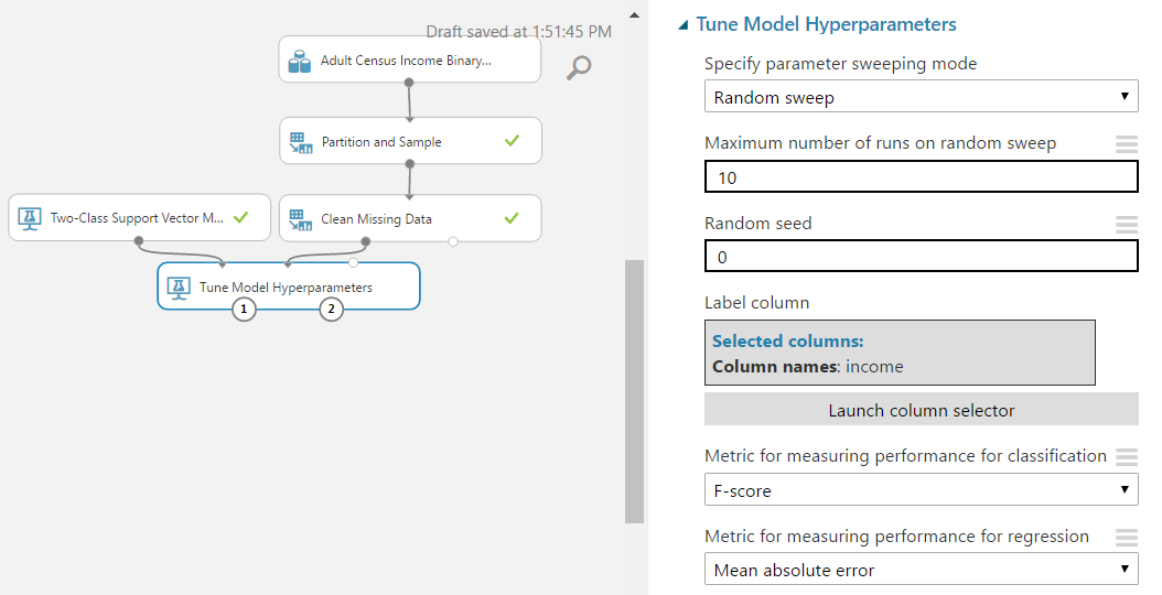
this. Let's use Tune Model Hyperparameters to find the best set of parameters for our Two-Class Support Vector Machine algorithm. If you want to learn more about Tune Model Hyperparameters, check out our previous
post.
 |
| Tune Model Hyperparameters |
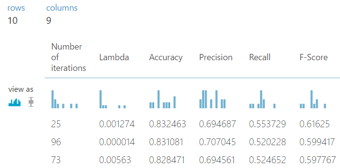
 |
| Tune Model Hyperparameters (Visualize) |
As you can see, the best model has 25 iterations with a Lambda of .001274. Let's plug that into our Two-Class Support Vector Machine algorithm and move on to Cross-Validation.
 |
| Cross Validate Model |
 |
| Contingency Table (Two-Class Averaged Perceptron) |
 |
| Contingency Table (Two-Class Boosted Decision Tree) |
 |
| Contingency Table (Two-Class Logistic Regression) |
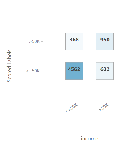
 |
| Contingency Table (Two-Class Support Vector Machine) |
As you can see, the Two-Class Support Vector Machine approach has about the same amount of True positives for "income = '<=50k'" as the rest of the models. However, the number of true positives for "income = '>50k'" is significantly less than that of the Two-Class Boosted Decision Tree. Therefore, using accuracy alone, we can say that the Two-Class Boosted Decision Tree model is the best model for this data.
We've mentioned a couple of times that there are more ways to measure "goodness" of a model besides Accuracy. In order to look at these, let's examine another module called "Evaluate Model".
 |
| Evaluate Model |
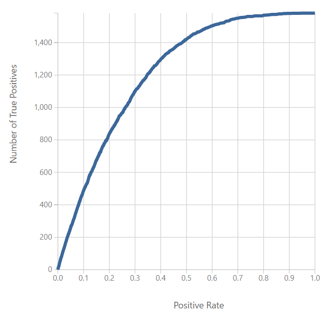
There are no parameters to set for the "Evaluate Model" module. All you do is provide it 1 or 2 scored datasets and it will provide a huge amount of information about the "goodness" of those models. Here's a snippet of what you can find.
 |
| Roc Curve |
 |
| Precision/Recall Curve |
 |
| Lift Curve |
The three charts shown above are the
ROC Curve,
Precision/Recall Curve, and
Lift Curve. We simply wanted to introduce these concepts to you in this post. We'll spend a lot more time talking about these metrics in a later post. Thanks for reading. We hope you found this informative.
Brad Llewellyn
Data Scientist
Valorem Consulting
@BreakingBI
www.linkedin.com/in/bradllewellyn
llewellyn.wb@gmail.com


No comments:
Post a Comment