Azure Machine Learning Workbench: Built-In Data Preparation, Part 1

Today, we're going to continue our walkthrough of the "Classifying_Iris" template provided as part of the AML Workbench.  Previously, we've look at Getting Started, Utilizing Different Environments and Built-In Data Sources.  In this post, we're going to focus on the built-in data preparation options that the AML Workbench provides.

Prepare Data

Let's start by navigating over to the "Data" pane and select the "Iris" Data Source.  From here, we have two options.  First, we could use an existing Data Preparation by selecting it from the "Data Preparations" list in the "Data" pane.  We also have the option of selecting the "Prepare" option at the top of "iris" tab.  This option will allow us to start from scratch.  Let's go with the second option for now.

Prepare

In the "Prepare" window, we need to choose with "Data Preparation Package" we want to use.  Basically, a Data Preparation Package is a grouping of transformations that are run as a unit.  This package will import all of the necessary data and run any number of transformations on any number of data sources, with only a single line of code.

Data Preparation

If we choose to use the existing iris.dprep package, we end up with a new tab that looks very similar to the Data Source tab, with a few additions.  On the left side of the tab, we have the "Dataflows" pane.  A Dataflow is a set of transformations performed on a single Data Source.  On the right side of the tab, we see the "Steps" pane.  A Step is a single transformation.  Therefore, we can see that multiple Steps are grouped into a single Dataflow and multiple Dataflows are grouped into a single Data Preparation Package.

Some of you may have noticed something strange about the table in the middle of the tab.  The columns suddenly have names, despite us never having supplied them.  We can even see these steps reflected in the "Steps" pane.  This is because we aren't looking at the Dataflow we just created.  Instead, we are looking at the existing Dataflow.  Our Dataflow is the second one on the list, with the identical name.

Empty Dataflow

If we select the second Dataflow in the "Dataflows" pane, we find our empty Dataflow.  In most cases, it's not very useful to have two different sets of transformations using the same data.  So, we'll throw away this Dataflow and use the one that's been provided to us.  However, it is important to note that it is possible to use the same Data Source multiple times within the same Data Preparation Package.

Remove Dataflow

Let's take a look at the existing Dataflow again.

Existing Dataflow

Steps Pane

The "Steps" pane shows us that three sets of transformation have been applied in this Dataflow.  First, the Dataflow was created.  Then, the column names were added since they did not exist in the original csv.  Finally, the Dataflow was filtered based on the "Species" column.  We can edit any of these steps by selecting the arrow next to them, then selecting "Edit".

Edit

Reference Dataflow

Rename Column

Filter Column

We can use these windows to see exactly what each step is doing and make any changes if we would like.

Step Options

Outside of editing the individual step, we also have the option of moving the step up or down in the Dataflow or deleting it entirely.  It's important to note that modifying steps further back in the Dataflow could potentially break steps that occur after it.  For instance, assume we are using column "A" in the calculation of column "B", then deleting column "A".  If we were to move the delete step before the calculation step, then the calculation of column "B" would break because column "A" no longer exists.

Halfway Complete

Another very important thing to notice about the "Steps" pane is that we can choose to look at the Dataflow after ANY number of steps.  For instance, if we select the "Rename Column3 to Petal Length" step, we can see the Dataflow as it looked after that step.  Notice that Column4 and Column5 have not been renamed yet.  Using this technique, we can add a new Step at this point, thereby adding it to the middle of the existing Dataflow.  This can be useful if we find that we missed a transformation along the line.

Inspectors

Let's finish by talking about "Inspectors".  Inspectors are nothing more than charts that give us a live view of our Dataflow.  We can see that we have a few different options to choose from.  More importantly, Inspectors are completely independent of Steps.  This means that we can create an Inspector to look at our data, then see how that particular data point changes with each step.  For instance, we have an Inspector that shows us the "Top 6 values of 'Species'".  If we move back to a step before the column "Species" existed, we see that this Inspector is no longer valid.  Obviously, this could be extremely helpful at examining the impact of certain filters or calculations.

No Species

There's way more to cover here than we have time for in this post.  Hopefully, this post opened your eyes to how easy it is to use the Built-In Data Preparation options in the Azure Machine Learning Workbench.  If you're eager to see more about Data Preparation in AML Workbench, read this.  Stay tuned for the next post where we'll be walking through some of the transformation options available in this extremely powerful tool.  Thanks for reading.  We hope you found this informative.

Brad Llewellyn
Senior Analytics Associate - Data Science
Syntelli Solutions
@BreakingBI
www.linkedin.com/in/bradllewellyn
llewellyn.wb@gmail.com

Azure Machine Learning Workbench: Built-In Data Sources

Today, we're going to continue our walkthrough of the "Classifying_Iris" template provided as part of the AML Workbench.  Previously, we've looked at Getting Started and Utilizing Different Environments.  In this post, we're going to focus on the built-in data source options that the AML Workbench provides.

Data

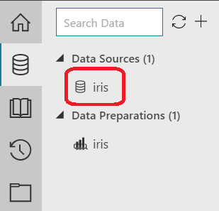
Let's start by opening the Data pane from the left side of the window.

Data Pane

Here, we have the option of selecting "Data Sources" or "Data Preparations".  "Data Sources" are what we use to bring our data in, as well perform some basic transformations to our data.  "Data Transformations" give us quite a few more options for transform and clean our data.  Additionally, we can have multiple "Data Transformations" using the same "Data Source".  This allows us to create separate datasets for testing different types of transformations or for creating different datasets entirely using the same base dataset.  Let's take a look at the "Data Source"

iris Data Source

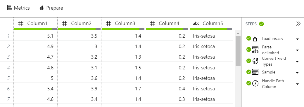
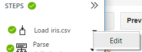
In this tab, we can see a few different areas.  First, we can see the result of our data import in tabular format.  This gives us a quick glance at what the data looks like.  On the right side of the screen, we can see the steps that were taken to generate this data source.  For those familiar with the Query Editor in Power BI (formerly known as Power Query), this is a very similar interface.  We can alter any of the steps by clicking on the arrow beside them and selecting "Edit".  Let's do this for the first step, "Load iris.csv".

Edit Data Source

Edit Data Source Path

In this situation, the only option is to edit the location of the Data Source.  You can read more about supported data formats here.

Despite its spreadsheet feel and list of applied steps, the "Data Source" section has very few options.  In fact, the steps we see utilized are ALL of the steps available.  We cannot do any data transformation or manipulation in this tab.  However, we do have an interesting option at the top of the tab called "Metrics".

Metrics

iris Metrics

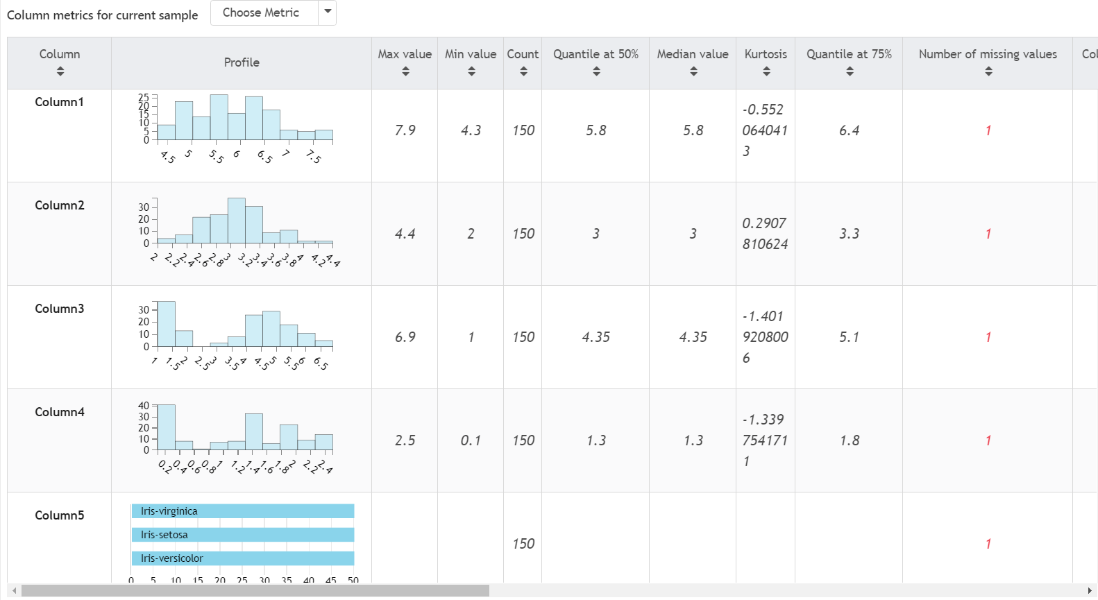
In this view, we can see a quick profile of the data (either a histogram or a bar chart based on the type of column), as well as a long list of metrics.  Here's a summary of the metrics provided.

Max Value: Largest Value in the Column

Min Value: Smallest Value in the Column

Count: Number of Records with Values in this column

Quantile at 50%: A measure of the "central" value in a dataset.  If the dataset was sorted, 50% of the values would be equal to or below this value.

Median: Same as Quantile at 50%

Kurtosis: Steepness of the distribution, i.e. a measure of the number of extreme observations it generates.

Quantile at 75%: If the dataset was sorted, 75% of the values would be equal to or below this value.

Number of Missing Values: Number of Records with No Value in this column

Column Data Type: The type of values that appears in the column.

Standard Deviation: Spread of the distribution, i.e. a measure of the distance between values in the column.

Variance: Spread of the distribution, i.e. a measure of the distance between values in the column., i.e. a measure of the distance between values in the column.  This is the square of the Standard Deviation.

Quantile at 25%: If the dataset was sorted, 25% of the values would be equal to or below this value.

Is Numeric Column: Whether the values in the columns are numbers and have the appropriate data type to match.

Number of NaNs: The number of records that contain values which are not numbers.  This does not consider the data type of the column and does not include missing values.

Mean Value: A measure of the "central" value in a dataset.  Calculated as the sum of all values in the column, divided by the number of values.  Commonly referred to as the "Average".

Unbiased Standard Error of the Mean: A measure of the stability of "Sample Mean" across samples.  If we assume our dataset is a sample of a larger distribution, then that distribution likely has a Mean.  However, since our sample is only part of the overall distribution, the mean of the sample will take different values based on which records are included in the sample.  Therefore, we can say that the sample mean has it's own distribution, known as a "Sampling Distribution".  This distribution likely has a standard deviation.  This is known as the "standard error of the sample mean".

Skewness: A measure of how NOT symmetric the distribution is, i.e. positive values signify the data has outliers larger than the mean, negative values signify the data has outliers smaller than the mean.

Most Common: The most common value in the column.  Commonly called the "Mode".  This only
applies to non-numeric columns.

Count of Most Common: The number of Records that contain the most common value.  This only applies to non-numeric columns.

Number of Unique Values: The number of distinct values within the column, i.e. every distinct value is counted only once, regardless of how many times it appears in the column.

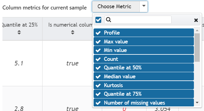
Metrics Filter

At the top of Metrics view, we also have the ability to filter the metrics we see.  This is a great way to get a view of only the information we are interested in.

Prepare (from Data view)

Prepare (from Metrics view)

At the top of the Data Source tab, regardless of whether we are looking at the Data or Metrics view, there's another option called "Prepare".  This will take us to the Data Preparations tab, which functions very similarly to the Query Editor in Power BI.  We'll cover this in the next post.

Instead of going through the rest of the options available for editing in the Data Sources tab, let's create a new data source to see it from scratch.  We've made a copy of the "iris.csv" file on our local machine.

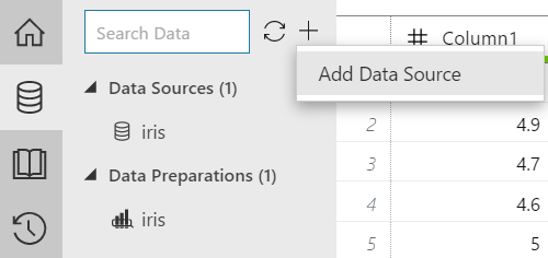
Add Data Source

At the top of the Data pane, we can click on the "+" button, then "Add Data Source".

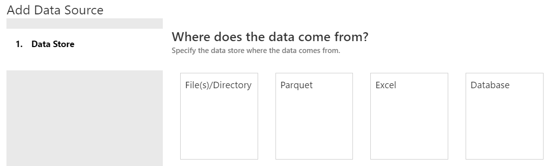
Data Store

On the next screen, we have the option of choosing where our data comes from.  We have a few different options.  We can read files from our local machine or blob storage.  We can read Parquet files from our local machine.  Parquet is an open-source columnar file format common with big data solutions.  You can read more about it here.  We can also read from Excel files in local or blob storage.  Finally, we can read from a SQL Server Database as well.  For more information on Data Sources, read this.  In our case, we want to pull from a csv on our local machine.  Therefore, we want to use the File(s)/Directory option.

File Selection

In the next tab, we select the file(s) that we want to import.  In our case, this is the "iris - Copy.csv" file from our local machine.

File Details 1

File Details 2

File Details 3

The next tab, "File Details" has some awkward scrolling.  So, we had to make some interesting screenshot decisions to capture everything.  On this tab, AML Workbench has already looked at the file and guessed at most of these properties.  However, if we want to, we can change them.  We get to define our File Type.  The options are "Delimited File", "Fixed-Width File", "Plain Text File" and "JSON File".  In our case, we want to use a "Delimited File" with a Separator of "Comma".  We also get to decide whether we want to skip the first few lines.  In our case we do not want to do this.  We can also choose our File Encoding.  There are a number of options here.  In our case, we want to use utf-8.  We can also let the tool know whether our file(s) have headers, i.e. column names.  In this case, we do not.  The last option is whether we want to handle Quoted Line Breaks.  Honestly, we have no idea what this means as we've never seen it before.  Perhaps someone in the comments can let us know.  Finally, we get to see the results of our selections at the bottom of the tab.

Data Types 1

Data Types 2

On the next tab, AML Workbench automatically detects data types.  However, it's always a good idea to check them in case we have to make some changes.  The built-in options are "Numeric", "Date", "Boolean" (TRUE/FALSE) and "String".  These options all look correct.  It's also important to notice that AML Workbench added a field to the front of our dataset called "Path".  Since we only used one file, this field is pretty worthless.  However, if we were to pull in files from a directory, this could be a great to determine which file a record came from.

Sampling

Depending on the size of the file, we may want to work with a sample to improve performance.  The available options are "Top N", "Full File", "Random N%" and "Random N", with a default of "Top 10,000".  Our file is small; so there's no harm in pulling in the full file.  As we see above, we can also create multiple sampling rules, then choose which one we want to be active.  This is an easy way to develop using a sample, then swap over to "Full File" when we're ready for full-scale testing.  Depending on your Python skills, you may also consider utilizing more complex sampling techniques later using a Python notebook.  We'll cover these in a later post.

Path Column

Finally, we get to choose whether we want to include the path column in our output data.  As we talked about earlier, there's no reason to include it in this case.

iris - Copy Data Source

Hopefully this post opened your eyes to the different possibilities for importing data into Azure Machine Learning Workbench.  This is an extremely powerful tool and we've only begun to scratch the surface.  Stay tuned for the next post where we'll walk through the Built-In Data Preparations.  Thanks for reading.  We hope you found this informative.

Brad Llewellyn
Senior Analytics Associate - Data Science
Syntelli Solutions
@BreakingBI
www.linkedin.com/in/bradllewellyn
llewellyn.wb@gmail.com

Azure Machine Learning Workbench: Utilizing Different Environments

Today, we're going to continue looking at the Azure Machine Learning (AML) Workbench.  In the previous post, we created a new Classifying_Iris project and walked through the basic layout of the Workbench.  In this post, we'll be walking through the rest of the code in the Quick CLI Reference section of the Dashboard.  This will focus on running our code utilizing different environments.

One of the biggest advantages of the cloud for modern data science is the ability to endlessly scale your resources in order to solve the problem at hand.  In some cases, like small-scale development, it's acceptable to run a process on our local machine.  However, as we need more processing power, we need to be able to run our code in more powerful environments, such as Azure Virtual Machines or HDInsight clusters.  Let's see how AML Workbench helps us accomplish this.

If you are new to the AML Workbench and haven't read the previous post, it is highly recommended that you do so.  The rest of this post will build on what we learned in the previous one.

Here's the first piece of code we will run.

az ml experiment submit -c local iris_sklearn.py

This code runs the "iris_sklearn.py" Python script using our local machine.  We'll cover exactly what this script does in a later post.  All we need to know for now is that it's running on our local machine using Python.  As we mentioned before, using the local machine is great if we're just trying to do something small without having to worry about connecting to remote resources.  Here's the output.

OUTPUT BEGIN

RunId: Classifying_Iris_1509458498714

Executing user inputs .....
===========================

Python version: 3.5.2 |Continuum Analytics, Inc.| (default, Jul  5 2016, 11:41:13) [MSC v.1900 64 bit (AMD64)]

Iris dataset shape: (150, 5)
Regularization rate is 0.01
LogisticRegression(C=100.0, class_weight=None, dual=False, fit_intercept=True,
          intercept_scaling=1, max_iter=100, multi_class='ovr', n_jobs=1,
          penalty='l2', random_state=None, solver='liblinear', tol=0.0001,
          verbose=0, warm_start=False)
Accuracy is 0.6792452830188679

==========================================
Serialize and deserialize using the outputs folder.

Export the model to model.pkl
Import the model from model.pkl
New sample: [[3.0, 3.6, 1.3, 0.25]]
Predicted class is ['Iris-setosa']
Plotting confusion matrix...
Confusion matrix in text:
[[50  0  0]
 [ 1 37 12]
 [ 0  4 46]]
Confusion matrix plotted.
Plotting ROC curve....
ROC curve plotted.
Confusion matrix and ROC curve plotted. See them in Run History details page.

Execution Details
=================

RunId: Classifying_Iris_1509458498714

OUTPUT END

Here's the next piece of code.

az ml experiment submit -c docker-python iris_sklearn.py

This code runs the same "iris_sklearn.py" script as before.  However, this time it uses a Python-enabled Docker container.  Docker is a technology that allows us package an entire environment into a single object.  This is extremely useful when we are trying to deploy code across distributed systems.  For instance, some organizations will wrap their applications in Docker containers, then deploy the Docker containers.  This allows them to manage the applications much easier because they can update the master Docker container, and that update can be automatically deployed to all of the existing Docker containers.  You can read more about Docker and containers here, here and here. Unfortunately, we're unable to install Docker on our machine.  So, we'll have to skip this one.  Let's take a look at the next piece of code.

az ml experiment submit -c docker-spark iris_pyspark.py

This code runs a new script called "iris_pyspark.py".  We'll save the in-depth analysis of the code for a later post.  To heavily summarize, PySpark is a way to harness the power of Spark's big data analytical functionality from within Python.  This can be extremely useful when we want to analyze or model big data problems without using a remote Spark cluster.  Let's take a look at the next piece of code.

az ml computetarget attach --name myvm --address <ip address or FQDN> --username <username> --password <pwd> --type remotedocker

az ml experiment prepare -c myvm

az ml experiment submit -c myvm iris_pyspark.py

This is where things start to get interesting.  Previously, we were running everything on our local machine.  This is great when data is small.  However, it becomes unusable when we need to point to larger data sources.  Fortunately, the AML Workbench allows us to attach to a remote virtual machine in cases where we need additional resources.

Another important thing to notice is that we were able to seemlessly run the same code on our local machine as we are running on the virtual machine.  This means that we can develop on small samples on our local machine, then effortlessly run the same code on a larger virtual machine when we want to test against a larger dataset.  This is exactly why containers are becoming so popular.  They make it effortless to move code from a less powerful environment, like a local machine, up to a more powerful one, like a large virtual machine.

Another advantage of this ability is that we can now manage resource costs by limiting virtual machine usage.  The entire team can share the same virtual machine, using it only when they need the extra power.  We can even turn the vm off when we aren't using it, saving even more money.  You can read more about Azure Virtual Machines here.

Let's move to the final piece of code.

az ml computetarget attach --name myhdi --address <ip address or FQDN of the head node> --username <username> --password <pwd> --type cluster

az ml experiment prepare -c myhdi

az ml experiment submit -c myhdi iris_pyspark.py

This code is expands on the same concepts as the previous one.  In some cases, we have very large resource needs.  In those cases, even a powerful virtual machine may not have enough juice.  For those cases, we can use containers to deploy to an Azure HDInsight cluster.  This will allow us to take the same code we ran on our local machine and execute it full-scale using the power of Hadoop.  You can read more about HDInsight clusters here.

This post has opened our eyes to the power and flexibility that the AML Workbench can provide.  While it's more complicated than using its AML Studio counterpart, the power and flexibility it provides via containers can make all the difference for some organizations.  Stay tuned for the next post where we'll walk through the built-in data preparation capabilities of the Azure Machine Learning Workbench.  Thanks for reading.  We hope you found this informative.

Brad Llewellyn
Data Science Consultant
Valorem
@BreakingBI
www.linkedin.com/in/bradllewellyn
llewellyn.wb@gmail.com

Azure Machine Learning Webinars

As some of you may know, we've been giving Azure Machine Learning presentations for about a year now.  As promised, we wanted to include links to the videos, as well as any supplemental material for the presentations.

Azure Machine Learning Studio: Making Data Science Easy(er)

https://www.youtube.com/watch?v=QMj_dL64xCA

There are no supplemental materials for this presentation.

Azure Machine Learning Studio: Four Tips from the Pros

https://www.youtube.com/watch?v=d25wmQ_dSQg

https://drive.google.com/open?id=12xodphzcK1Oy7TBDDSzHPXe8GIiBIgbr

R Code for Creating Interaction Features

<R CODE START>

#####################

## Import Data

#####################

ignore <- c("income")

dat1 <- maml.mapInputPort(1)

dat.full <- dat1[,-which(names(dat1) %in% ignore)]

dat2 <- maml.mapInputPort(2)

vars.dummy <- names(dat.full)

vars.orig <- names(dat2[,-which(names(dat2) %in% ignore)])

temp <- dat.full[,1]

dat.int <- data.frame(temp)

################################################

## Loop through all possible combinations

################################################

for(i in 1:(length(vars.dummy) - 1)){

    for(j in 2:length(vars.dummy)){

        var1 <- vars.dummy[i]

        var2 <- vars.dummy[j]

        

        base1 <- substr(var1, 1, regexpr("-", var1) - 1)

        base2 <- substr(var2, 1, regexpr("-", var2) - 1)

        

        if( base1 != base2 ){

            val1 <- dat.full[,which(names(dat.full) %in% var1)]

            val2 <- dat.full[,which(names(dat.full) %in% var2)]

            dat.int[,length(dat.int) + 1] <- val1 * val2

            names(dat.int)[length(dat.int)] <- paste(var1, " * ", var2)

        }

    }

}

###################

## Output Data

###################

dat.out <- data.frame(dat1, dat.int[,-1])

maml.mapOutputPort("dat.out");

<R CODE END>

SQL Code for Combining Tune Model Hyperparameters Results

<SQL CODE 1 START>

SELECT
    'Two-Class Locally Deep Support Vector Machine - Binning' AS [Model Type]
,'LD-SVM Tree Depth' AS [Par 1 Name]
,[LD-SVM Tree Depth] AS [Par 1 Value]
,'Lambda W' AS [Par 2 Name]
,[Lambda W] AS [Par 2 Value]
,'Lambda Theta' AS [Par 3 Name]
,[Lambda Theta] AS [Par 3 Value]
,'Lambda Theta Prime' AS [Par 4 Name]
,[Lambda Theta Prime] AS [Par 4 Value]
,'Sigma' AS [Par 5 Name]
,[Sigma] AS [Par 5 Value]
,'Num Iterations' AS [Par 6 Name]
,[Num Iterations] AS [Par 6 Value]
    ,'None' AS [Par 7 Name]
    ,'' AS [Par 7 Value]
,[Accuracy]
,[Precision]
,[Recall]
,[F-Score]
,[AUC]
,[Average Log Loss]
,[Training Log Loss]
,[Precision] * [Recall] AS [Precision * Recall]
FROM t1
UNION ALL
SELECT
'Two-Class Neural Network - Binning' AS [Model Type]
,'Learning rate' AS [Par 1 Name]
,[Learning rate] AS [Par 1 Value]
    ,'None' AS [Par 2 Name]
    ,0 AS [Par 2 Value]
,'Number of iterations' AS [Par 3 Name]
,[Number of iterations] AS [Par 3 Value]
,'None' AS [Par 4 Name]
,0 AS [Par 4 Value]
,'None' AS [Par 5 Name]
,0 AS [Par 5 Value]
,'None' AS [Par 6 Name]
,0 AS [Par 6 Value]
,'LossFunction' AS [Par 7 Name]
,[LossFunction] AS [Par 7 Value]
,[Accuracy]
,[Precision]
,[Recall]
,[F-Score]
,[AUC]
,[Average Log Loss]
,[Training Log Loss]
,[Precision] * [Recall] AS [Precision * Recall]
FROM t2
UNION ALL
SELECT
'Two-Class Decision Jungle - Replicate' AS [Model Type]
,'Number of optimization steps per decision DAG layer' AS [Par 1 Name]
,[Number of optimization steps per decision DAG layer] AS [Par 1 Value]
,'Maximum width of the decision DAGs' AS [Par 2 Name]
,[Maximum width of the decision DAGs] AS [Par 2 Value]
,'Maximum depth of the decision DAGs' AS [Par 3 Name]
,[Maximum depth of the decision DAGs] AS [Par 3 Value]
,'Number of decision DAGs' AS [Par 4 Name]
,[Number of decision DAGs] AS [Par 4 Value]
,'None' AS [Par 5 Name]
,0 AS [Par 5 Value]
,'None' AS [Par 6 Name]
,0 AS [Par 6 Value]
    ,'None' AS [Par 7 Name]
    ,'' AS [Par 7 Value]
,[Accuracy]
,[Precision]
,[Recall]
,[F-Score]
,[AUC]
,[Average Log Loss]
,[Training Log Loss]
,[Precision] * [Recall] AS [Precision * Recall]

FROM t3

<SQL CODE 1 END>


<SQL CODE 2 START>

SELECT
'Two-Class Locally Deep Support Vector Machine - Gaussian' AS [Model Type]
,'LD-SVM Tree Depth' AS [Par 1 Name]
,[LD-SVM Tree Depth] AS [Par 1 Value]
,'Lambda W' AS [Par 2 Name]
,[Lambda W] AS [Par 2 Value]
,'Lambda Theta' AS [Par 3 Name]
,[Lambda Theta] AS [Par 3 Value]
,'Lambda Theta Prime' AS [Par 4 Name]
,[Lambda Theta Prime] AS [Par 4 Value]
,'Sigma' AS [Par 5 Name]
,[Sigma] AS [Par 5 Value]
,'Num Iterations' AS [Par 6 Name]
,[Num Iterations] AS [Par 6 Value]
    ,'None' AS [Par 7 Name]
    ,'' AS [Par 7 Value]
,[Accuracy]
,[Precision]
,[Recall]
,[F-Score]
,[AUC]
,[Average Log Loss]
,[Training Log Loss]
,[Precision] * [Recall] AS [Precision * Recall]
FROM t1
UNION ALL
SELECT
'Two-Class Neural Network - Gaussian' AS [Model Type]
,'Learning rate' AS [Par 1 Name]
,[Learning rate] AS [Par 1 Value]
    ,'None' AS [Par 2 Name]
    ,0 AS [Par 2 Value]
,'Number of iterations' AS [Par 3 Name]
,[Number of iterations] AS [Par 3 Value]
,'None' AS [Par 4 Name]
,0 AS [Par 4 Value]
,'None' AS [Par 5 Name]
,0 AS [Par 5 Value]
,'None' AS [Par 6 Name]
,0 AS [Par 6 Value]
,'LossFunction' AS [Par 7 Name]
,[LossFunction] AS [Par 7 Value]
,[Accuracy]
,[Precision]
,[Recall]
,[F-Score]
,[AUC]
,[Average Log Loss]
,[Training Log Loss]
,[Precision] * [Recall] AS [Precision * Recall]
FROM t2
UNION ALL
SELECT
'Two-Class Decision Jungle - Bagging' AS [Model Type]
,'Number of optimization steps per decision DAG layer' AS [Par 1 Name]
,[Number of optimization steps per decision DAG layer] AS [Par 1 Value]
,'Maximum width of the decision DAGs' AS [Par 2 Name]
,[Maximum width of the decision DAGs] AS [Par 2 Value]
,'Maximum depth of the decision DAGs' AS [Par 3 Name]
,[Maximum depth of the decision DAGs] AS [Par 3 Value]
,'Number of decision DAGs' AS [Par 4 Name]
,[Number of decision DAGs] AS [Par 4 Value]
,'None' AS [Par 5 Name]
,0 AS [Par 5 Value]
,'None' AS [Par 6 Name]
,0 AS [Par 6 Value]
    ,'None' AS [Par 7 Name]
    ,'' AS [Par 7 Value]
,[Accuracy]
,[Precision]
,[Recall]
,[F-Score]
,[AUC]
,[Average Log Loss]
,[Training Log Loss]
,[Precision] * [Recall] AS [Precision * Recall]

FROM t3

<SQL CODE 2 END>


<SQL CODE 3 START>

SELECT
'Two-Class Locally Deep Support Vector Machine - Min-Max' AS [Model Type]
,'LD-SVM Tree Depth' AS [Par 1 Name]
,[LD-SVM Tree Depth] AS [Par 1 Value]
,'Lambda W' AS [Par 2 Name]
,[Lambda W] AS [Par 2 Value]
,'Lambda Theta' AS [Par 3 Name]
,[Lambda Theta] AS [Par 3 Value]
,'Lambda Theta Prime' AS [Par 4 Name]
,[Lambda Theta Prime] AS [Par 4 Value]
,'Sigma' AS [Par 5 Name]
,[Sigma] AS [Par 5 Value]
,'Num Iterations' AS [Par 6 Name]
,[Num Iterations] AS [Par 6 Value]
    ,'None' AS [Par 7 Name]
    ,'' AS [Par 7 Value]
,[Accuracy]
,[Precision]
,[Recall]
,[F-Score]
,[AUC]
,[Average Log Loss]
,[Training Log Loss]
,[Precision] * [Recall] AS [Precision * Recall]
FROM t1
UNION ALL
SELECT
'Two-Class Neural Network - Min-Max' AS [Model Type]
,'Learning rate' AS [Par 1 Name]
,[Learning rate] AS [Par 1 Value]
,'None' AS [Par 2 Name]
,0 AS [Par 2 Value]
,'Number of iterations' AS [Par 3 Name]
,[Number of iterations] AS [Par 3 Value]
,'None' AS [Par 4 Name]
,0 AS [Par 4 Value]
,'None' AS [Par 5 Name]
,0 AS [Par 5 Value]
,'None' AS [Par 6 Name]
,0 AS [Par 6 Value]
,'LossFunction' AS [Par 7 Name]
,[LossFunction] AS [Par 7 Value]
,[Accuracy]
,[Precision]
,[Recall]
,[F-Score]
,[AUC]
,[Average Log Loss]
,[Training Log Loss]
,[Precision] * [Recall] AS [Precision * Recall]
FROM t2
UNION ALL
SELECT
'Two-Class Boosted Decision Tree' AS [Model Type]
,'Number of leaves' AS [Par 1 Name]
,[Number of leaves] AS [Par 1 Value]
,'Minimum leaf instances' AS [Par 2 Name]
,[Minimum leaf instances] AS [Par 2 Value]
,'Learning rate' AS [Par 3 Name]
,[Learning rate] AS [Par 3 Value]
,'Number of trees' AS [Par 4 Name]
,[Number of trees] AS [Par 4 Value]
,'None' AS [Par 5 Name]
,0 AS [Par 5 Value]
,'None' AS [Par 6 Name]
,0 AS [Par 6 Value]
    ,'None' AS [Par 7 Name]
    ,'' AS [Par 7 Value]
,[Accuracy]
,[Precision]
,[Recall]
,[F-Score]
,[AUC]
,[Average Log Loss]
,[Training Log Loss]
,[Precision] * [Recall] AS [Precision * Recall]

FROM t3

<SQL CODE 3 END>


<SQL CODE 4 START>

SELECT
'Two-Class Decision Forest - Replicate' AS [Model Type]
,'Minimum number of samples per leaf node' AS [Par 1 Name]
,[Minimum number of samples per leaf node] AS [Par 1 Value]
,'Number of random splits per node' AS [Par 2 Name]
,[Number of random splits per node] AS [Par 2 Value]
,'Maximum depth of the decision trees' AS [Par 3 Name]
,[Maximum depth of the decision trees] AS [Par 3 Value]
,'Number of decision trees' AS [Par 4 Name]
,[Number of decision trees] AS [Par 4 Value]
,'None' AS [Par 5 Name]
,0 AS [Par 5 Value]
,'None' AS [Par 6 Name]
,0 AS [Par 6 Value]
    ,'None' AS [Par 7 Name]
    ,'' AS [Par 7 Value]
,[Accuracy]
,[Precision]
,[Recall]
,[F-Score]
,[AUC]
,[Average Log Loss]
,[Training Log Loss]
,[Precision] * [Recall] AS [Precision * Recall]
FROM t1
UNION ALL
SELECT
'Two-Class Averaged Perceptron' AS [Model Type]
,'Learning rate' AS [Par 1 Name]
,[Learning rate] AS [Par 1 Value]
,'Maximum number of iterations' AS [Par 2 Name]
,[Maximum number of iterations] AS [Par 2 Value]
,'None' AS [Par 3 Name]
,0 AS [Par 3 Value]
,'None' AS [Par 4 Name]
,0 AS [Par 4 Value]
,'None' AS [Par 5 Name]
,0 AS [Par 5 Value]
,'None' AS [Par 6 Name]
,0 AS [Par 6 Value]
    ,'None' AS [Par 7 Name]
    ,'' AS [Par 7 Value]
,[Accuracy]
,[Precision]
,[Recall]
,[F-Score]
,[AUC]
,[Average Log Loss]
,[Training Log Loss]
,[Precision] * [Recall] AS [Precision * Recall]
FROM t2
UNION ALL
SELECT
'Two-Class Support Vector Machine' AS [Model Type]
,'Number of iterations' AS [Par 1 Name]
,[Number of iterations] AS [Par 1 Value]
,'Lambda' AS [Par 2 Name]
,[Lambda] AS [Par 2 Value]
,'None' AS [Par 3 Name]
,0 AS [Par 3 Value]
,'None' AS [Par 4 Name]
,0 AS [Par 4 Value]
,'None' AS [Par 5 Name]
,0 AS [Par 5 Value]
,'None' AS [Par 6 Name]
,0 AS [Par 6 Value]
    ,'None' AS [Par 7 Name]
    ,'' AS [Par 7 Value]
,[Accuracy]
,[Precision]
,[Recall]
,[F-Score]
,[AUC]
,[Average Log Loss]
,[Training Log Loss]
,[Precision] * [Recall] AS [Precision * Recall]

FROM t3

<SQL CODE 4 END>


<SQL CODE 5 START>

SELECT
'Two-Class Decision Forest - Bagging' AS [Model Type]
,'Minimum number of samples per leaf node' AS [Par 1 Name]
,[Minimum number of samples per leaf node] AS [Par 1 Value]
,'Number of random splits per node' AS [Par 2 Name]
,[Number of random splits per node] AS [Par 2 Value]
,'Maximum depth of the decision trees' AS [Par 3 Name]
,[Maximum depth of the decision trees] AS [Par 3 Value]
,'Number of decision trees' AS [Par 4 Name]
,[Number of decision trees] AS [Par 4 Value]
,'None' AS [Par 5 Name]
,0 AS [Par 5 Value]
,'None' AS [Par 6 Name]
,0 AS [Par 6 Value]
    ,'None' AS [Par 7 Name]
    ,'' AS [Par 7 Value]
,[Accuracy]
,[Precision]
,[Recall]
,[F-Score]
,[AUC]
,[Average Log Loss]
,[Training Log Loss]
,[Precision] * [Recall] AS [Precision * Recall]
FROM t1
UNION ALL
SELECT
'Two-Class Logistic Regression' AS [Model Type]
,'OptimizationTolerance' AS [Par 1 Name]
,[OptimizationTolerance] AS [Par 1 Value]
,'L1Weight' AS [Par 2 Name]
,[L1Weight] AS [Par 2 Value]
,'L2Weight' AS [Par 3 Name]
,[L2Weight] AS [Par 3 Value]
,'MemorySize' AS [Par 4 Name]
,[MemorySize] AS [Par 4 Value]
,'None' AS [Par 5 Name]
,0 AS [Par 5 Value]
,'None' AS [Par 6 Name]
,0 AS [Par 6 Value]
    ,'None' AS [Par 7 Name]
    ,'' AS [Par 7 Value]
,[Accuracy]
,[Precision]
,[Recall]
,[F-Score]
,[AUC]
,[Average Log Loss]
,[Training Log Loss]
,[Precision] * [Recall] AS [Precision * Recall]

FROM t2

<SQL CODE 5 END>


<SQL CODE 6 START>

SELECT * FROM t1
UNION ALL
SELECT * FROM t2
UNION ALL

SELECT * FROM t3

<SQL CODE 6 END>


<SQL CODE 7 START>

SELECT * FROM t1
UNION ALL

SELECT * FROM t2

<SQL CODE 7 END>


<SQL CODE 8 START>

SELECT * FROM t1
UNION ALL

SELECT * FROM t2

<SQL CODE 8 END>

<SQL CODE 9 START>

SELECT * FROM t1
ORDER BY [AUC] DESC

<SQL CODE 9 END>

Brad Llewellyn
Data Science Consultant
Valorem
@BreakingBI
www.linkedin.com/in/bradllewellyn
llewellyn.wb@gmail.com

Azure Machine Learning Workbench: Getting Started

Today, we're going to take a look at one of the newest Data Science offerings from Microsoft.  Of course, we're talking about the Azure Machine Learning (AML) Workbench!  Join us as we dive in and see what this new tool is all about.

Before we install the AML Workbench, let's talk about what it is.  The AML Workbench is a local environment for developing data science solutions that can be easily deployed and managed using Microsoft Azure.  It doesn't appear to be related to AML Studio in any way.  Throughout this series, we'll walk through all of the different things we can do with the AML Workbench.  For today, we're just going to get our feet wet.

Now, we need to create an Azure Machine Learning Experimentation resource in the Azure portal.  You can find complete instructions here.  We will also include a Workspace and a Model Management Account.  This appears to be free for the first two users.  However, we're not sure whether they charge separately for the storage account.  Maybe someone can let us know in the comments.  Now, let's boot this baby up!

Azure Machine Learning Workbench

New Project

In the top-left corner, we can see the Workspace we created in the Azure portal.  Let's add a new Project to this.

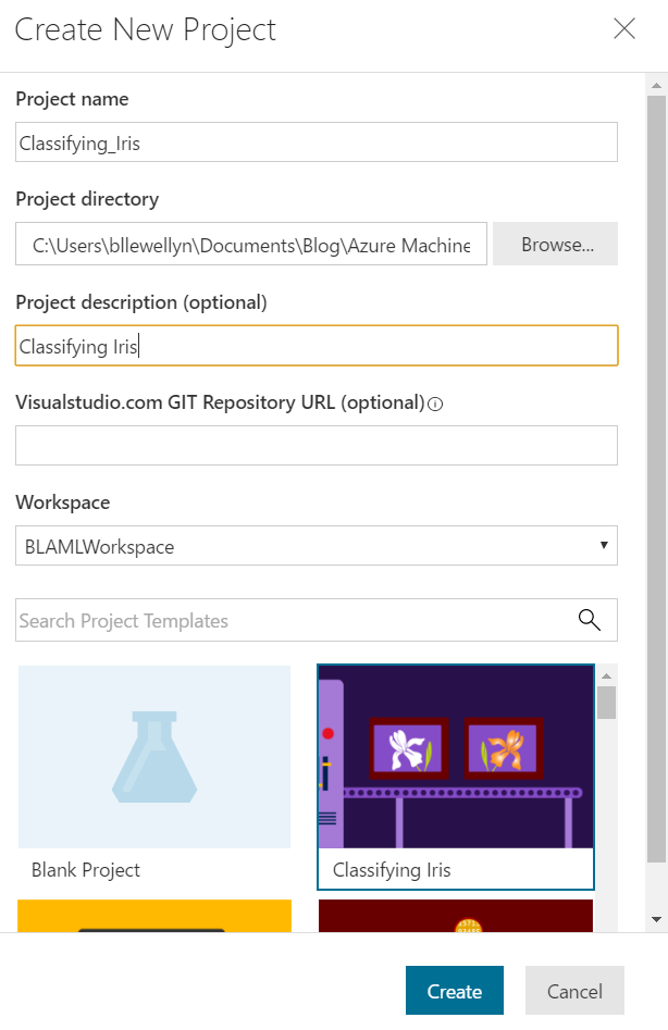
Create New Project

Now, we have to add the details for our new project.  Strangely, the project name can't include spaces.  We felt like we were past the point where names had to be simple, but maybe it's a Git thing.  Either way, we'll call our new project "Classifying_Iris" and use the "Classifying Iris" template at the bottom of the screen.  Let's see what's inside this project.

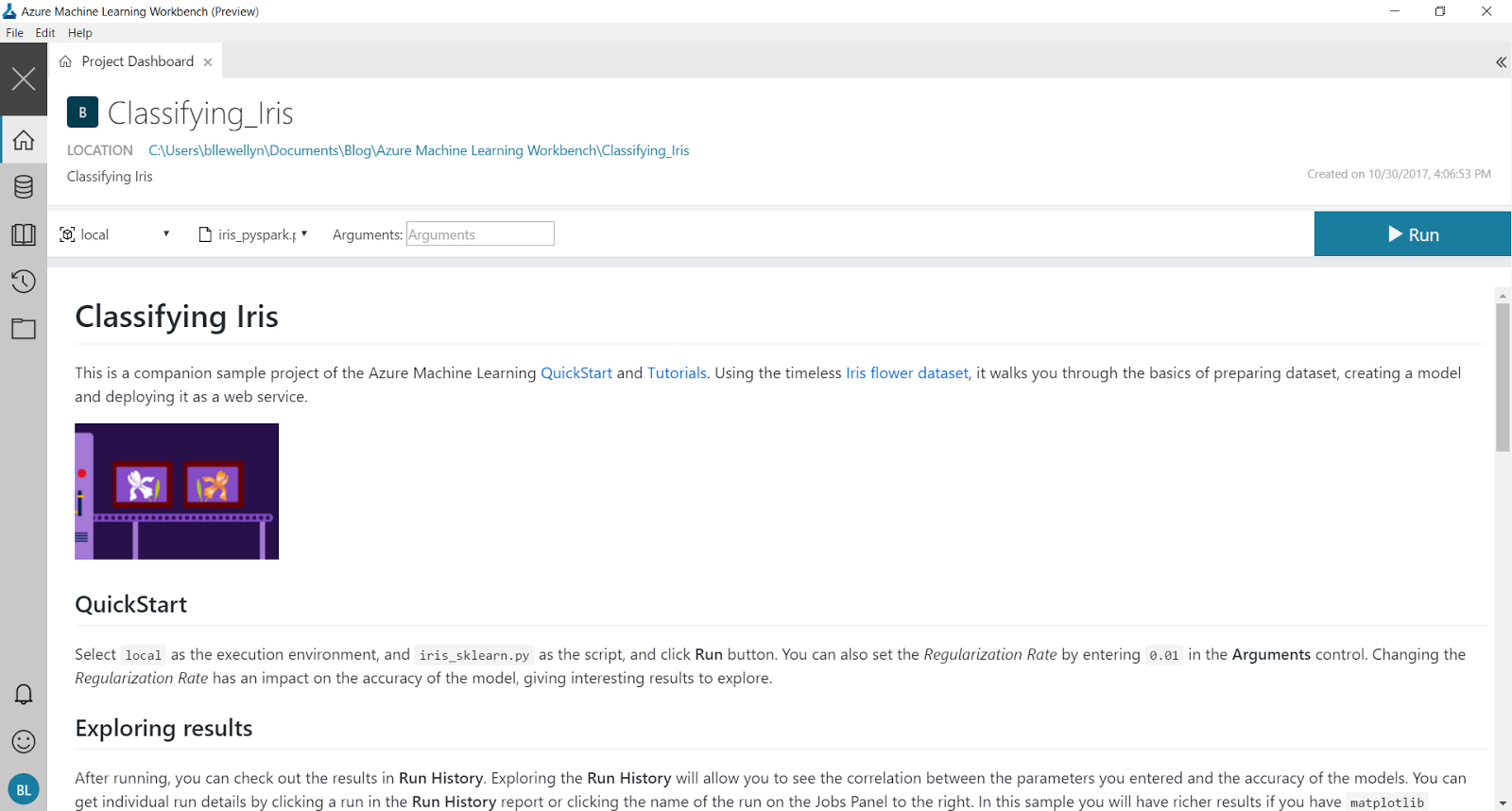
Project Dashboard

The first thing we see is the Project Dashboard.  This is a great place to create (or read) quality documentation on exactly what the project does, links to external resources, etc.

iris_sklearn

Following the QuickStart instructions, we were able to run the "iris_sklearn.py" code.  Unfortunately, it's not immediately obvious what this does.  Fortunately, the Exploring Results section tells us to check the Run History.  We can find this icon on the left side of the screen.

Run History

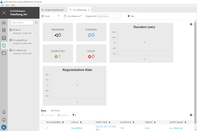
iris_sklearn Run History

This is pretty cool stuff actually.  This view would let us know how long our code is taking to run, as well as what parameters are being input.  This would be extremely helpful if we were running repeated experiments.  In our case, it doesn't show much though.

Job History

If we click on the Job Name in the Jobs section on the right side of the screen, we can see a more detailed result set.

Run Properties

This is what we were looking for!  This gives us all kinds of information about the run.  This could be extremely useful for showing the results of an experiment to bosses or colleagues.

Logs

Further down the page, we see the Logs section.  This is where we can access all the granular information we would need if we needed to debug a particular issue.

The next section of the instructions is the Quick CLI Reference.  This gives us a bunch of code we can use to run these scripts from the Command Line (or Powershell).  Let's open a new command line window.

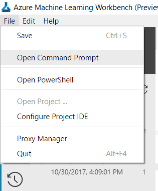
Open Command Prompt

In the top-left corner of the window, we can select "Open Command Prompt" from the "File" menu.

Command Prompt

In the command prompt, we can copy the first line of code from the instructions.

pip install matplotlib

This code will install the Python library "matplotlib".  This library contains quite a few functions for creating graphs in Python.  You can read more about it here.  Now that we have the library installed, let's copy the next line of code.

az login

This code will help us log the Command Line Interface into Azure.  When we run this command, we get the following response.

To sign in, use a web browser to open the page https://aka.ms/devicelogin and enter the code ######### to authenticate.

When we follow the instructions, we can log into our Azure subscription.

Azure Login

The next piece of code we need to run is as follows.

python run.py

This piece of code will run the "run.py" script from our project.  We'll look at this script in a later post.  For now, let's see the output from this script.  Please note that the "run.py" script is iterative and creates a large amount of output.  You can skip to the OUTPUT END header if you don't want to see the output.

OUTPUT BEGIN

RunId: Classifying_Iris_1509457170414

Executing user inputs .....
===========================

Python version: 3.5.2 |Continuum Analytics, Inc.| (default, Jul  5 2016, 11:41:13) [MSC v.1900 64 bit (AMD64)]

Iris dataset shape: (150, 5)
Regularization rate is 10.0
LogisticRegression(C=0.1, class_weight=None, dual=False, fit_intercept=True,
          intercept_scaling=1, max_iter=100, multi_class='ovr', n_jobs=1,
          penalty='l2', random_state=None, solver='liblinear', tol=0.0001,
          verbose=0, warm_start=False)
Accuracy is 0.6415094339622641

==========================================
Serialize and deserialize using the outputs folder.

Export the model to model.pkl
Import the model from model.pkl
New sample: [[3.0, 3.6, 1.3, 0.25]]
Predicted class is ['Iris-setosa']
Plotting confusion matrix...
Confusion matrix in text:
[[50  0  0]
 [ 0 31 19]
 [ 0  4 46]]
Confusion matrix plotted.
Plotting ROC curve....
ROC curve plotted.
Confusion matrix and ROC curve plotted. See them in Run History details page.

Execution Details
=================
RunId: Classifying_Iris_1509457170414

RunId: Classifying_Iris_1509457188739

Executing user inputs .....
===========================

Python version: 3.5.2 |Continuum Analytics, Inc.| (default, Jul  5 2016, 11:41:13) [MSC v.1900 64 bit (AMD64)]

Iris dataset shape: (150, 5)
Regularization rate is 5.0
LogisticRegression(C=0.2, class_weight=None, dual=False, fit_intercept=True,
          intercept_scaling=1, max_iter=100, multi_class='ovr', n_jobs=1,
          penalty='l2', random_state=None, solver='liblinear', tol=0.0001,
          verbose=0, warm_start=False)
Accuracy is 0.6415094339622641

==========================================
Serialize and deserialize using the outputs folder.

Export the model to model.pkl
Import the model from model.pkl
New sample: [[3.0, 3.6, 1.3, 0.25]]
Predicted class is ['Iris-setosa']
Plotting confusion matrix...
Confusion matrix in text:
[[50  0  0]
 [ 0 32 18]
 [ 0  4 46]]
Confusion matrix plotted.
Plotting ROC curve....
ROC curve plotted.
Confusion matrix and ROC curve plotted. See them in Run History details page.

Execution Details
=================
RunId: Classifying_Iris_1509457188739

RunId: Classifying_Iris_1509457195895

Executing user inputs .....
===========================

Python version: 3.5.2 |Continuum Analytics, Inc.| (default, Jul  5 2016, 11:41:13) [MSC v.1900 64 bit (AMD64)]

Iris dataset shape: (150, 5)
Regularization rate is 2.5
LogisticRegression(C=0.4, class_weight=None, dual=False, fit_intercept=True,
          intercept_scaling=1, max_iter=100, multi_class='ovr', n_jobs=1,
          penalty='l2', random_state=None, solver='liblinear', tol=0.0001,
          verbose=0, warm_start=False)
Accuracy is 0.660377358490566

==========================================
Serialize and deserialize using the outputs folder.

Export the model to model.pkl
Import the model from model.pkl
New sample: [[3.0, 3.6, 1.3, 0.25]]
Predicted class is ['Iris-setosa']
Plotting confusion matrix...
Confusion matrix in text:
[[50  0  0]
 [ 0 33 17]
 [ 0  4 46]]
Confusion matrix plotted.
Plotting ROC curve....
ROC curve plotted.
Confusion matrix and ROC curve plotted. See them in Run History details page.

Execution Details
=================
RunId: Classifying_Iris_1509457195895

RunId: Classifying_Iris_1509457203051

Executing user inputs .....
===========================

Python version: 3.5.2 |Continuum Analytics, Inc.| (default, Jul  5 2016, 11:41:13) [MSC v.1900 64 bit (AMD64)]

Iris dataset shape: (150, 5)
Regularization rate is 1.25
LogisticRegression(C=0.8, class_weight=None, dual=False, fit_intercept=True,
          intercept_scaling=1, max_iter=100, multi_class='ovr', n_jobs=1,
          penalty='l2', random_state=None, solver='liblinear', tol=0.0001,
          verbose=0, warm_start=False)
Accuracy is 0.6415094339622641

==========================================
Serialize and deserialize using the outputs folder.

Export the model to model.pkl
Import the model from model.pkl
New sample: [[3.0, 3.6, 1.3, 0.25]]
Predicted class is ['Iris-setosa']
Plotting confusion matrix...
Confusion matrix in text:
[[50  0  0]
 [ 1 33 16]
 [ 0  5 45]]
Confusion matrix plotted.
Plotting ROC curve....
ROC curve plotted.
Confusion matrix and ROC curve plotted. See them in Run History details page.

Execution Details
=================
RunId: Classifying_Iris_1509457203051

RunId: Classifying_Iris_1509457210237

Executing user inputs .....
===========================

Python version: 3.5.2 |Continuum Analytics, Inc.| (default, Jul  5 2016, 11:41:13) [MSC v.1900 64 bit (AMD64)]

Iris dataset shape: (150, 5)
Regularization rate is 0.625
LogisticRegression(C=1.6, class_weight=None, dual=False, fit_intercept=True,
          intercept_scaling=1, max_iter=100, multi_class='ovr', n_jobs=1,
          penalty='l2', random_state=None, solver='liblinear', tol=0.0001,
          verbose=0, warm_start=False)
Accuracy is 0.660377358490566

==========================================
Serialize and deserialize using the outputs folder.

Export the model to model.pkl
Import the model from model.pkl
New sample: [[3.0, 3.6, 1.3, 0.25]]
Predicted class is ['Iris-setosa']
Plotting confusion matrix...
Confusion matrix in text:
[[50  0  0]
 [ 1 36 13]
 [ 0  5 45]]
Confusion matrix plotted.
Plotting ROC curve....
ROC curve plotted.
Confusion matrix and ROC curve plotted. See them in Run History details page.

Execution Details
=================
RunId: Classifying_Iris_1509457210237

RunId: Classifying_Iris_1509457217482

Executing user inputs .....
===========================

Python version: 3.5.2 |Continuum Analytics, Inc.| (default, Jul  5 2016, 11:41:13) [MSC v.1900 64 bit (AMD64)]

Iris dataset shape: (150, 5)
Regularization rate is 0.3125
LogisticRegression(C=3.2, class_weight=None, dual=False, fit_intercept=True,
          intercept_scaling=1, max_iter=100, multi_class='ovr', n_jobs=1,
          penalty='l2', random_state=None, solver='liblinear', tol=0.0001,
          verbose=0, warm_start=False)
Accuracy is 0.660377358490566

==========================================
Serialize and deserialize using the outputs folder.

Export the model to model.pkl
Import the model from model.pkl
New sample: [[3.0, 3.6, 1.3, 0.25]]
Predicted class is ['Iris-setosa']
Plotting confusion matrix...
Confusion matrix in text:
[[50  0  0]
 [ 1 36 13]
 [ 0  4 46]]
Confusion matrix plotted.
Plotting ROC curve....
ROC curve plotted.
Confusion matrix and ROC curve plotted. See them in Run History details page.

Execution Details
=================
RunId: Classifying_Iris_1509457217482

RunId: Classifying_Iris_1509457225704

Executing user inputs .....
===========================

Python version: 3.5.2 |Continuum Analytics, Inc.| (default, Jul  5 2016, 11:41:13) [MSC v.1900 64 bit (AMD64)]

Iris dataset shape: (150, 5)
Regularization rate is 0.15625
LogisticRegression(C=6.4, class_weight=None, dual=False, fit_intercept=True,
          intercept_scaling=1, max_iter=100, multi_class='ovr', n_jobs=1,
          penalty='l2', random_state=None, solver='liblinear', tol=0.0001,
          verbose=0, warm_start=False)
Accuracy is 0.6792452830188679

==========================================
Serialize and deserialize using the outputs folder.

Export the model to model.pkl
Import the model from model.pkl
New sample: [[3.0, 3.6, 1.3, 0.25]]
Predicted class is ['Iris-setosa']
Plotting confusion matrix...
Confusion matrix in text:
[[50  0  0]
 [ 1 36 13]
 [ 0  3 47]]
Confusion matrix plotted.
Plotting ROC curve....
ROC curve plotted.
Confusion matrix and ROC curve plotted. See them in Run History details page.

Execution Details
=================
RunId: Classifying_Iris_1509457225704

RunId: Classifying_Iris_1509457234132

Executing user inputs .....
===========================

Python version: 3.5.2 |Continuum Analytics, Inc.| (default, Jul  5 2016, 11:41:13) [MSC v.1900 64 bit (AMD64)]

Iris dataset shape: (150, 5)
Regularization rate is 0.078125
LogisticRegression(C=12.8, class_weight=None, dual=False, fit_intercept=True,
          intercept_scaling=1, max_iter=100, multi_class='ovr', n_jobs=1,
          penalty='l2', random_state=None, solver='liblinear', tol=0.0001,
          verbose=0, warm_start=False)
Accuracy is 0.6792452830188679

==========================================
Serialize and deserialize using the outputs folder.

Export the model to model.pkl
Import the model from model.pkl
New sample: [[3.0, 3.6, 1.3, 0.25]]
Predicted class is ['Iris-setosa']
Plotting confusion matrix...
Confusion matrix in text:
[[50  0  0]
 [ 1 36 13]
 [ 0  3 47]]
Confusion matrix plotted.
Plotting ROC curve....
ROC curve plotted.
Confusion matrix and ROC curve plotted. See them in Run History details page.

Execution Details
=================
RunId: Classifying_Iris_1509457234132

RunId: Classifying_Iris_1509457242301

Executing user inputs .....
===========================

Python version: 3.5.2 |Continuum Analytics, Inc.| (default, Jul  5 2016, 11:41:13) [MSC v.1900 64 bit (AMD64)]

Iris dataset shape: (150, 5)
Regularization rate is 0.0390625
LogisticRegression(C=25.6, class_weight=None, dual=False, fit_intercept=True,
          intercept_scaling=1, max_iter=100, multi_class='ovr', n_jobs=1,
          penalty='l2', random_state=None, solver='liblinear', tol=0.0001,
          verbose=0, warm_start=False)
Accuracy is 0.6981132075471698

==========================================
Serialize and deserialize using the outputs folder.

Export the model to model.pkl
Import the model from model.pkl
New sample: [[3.0, 3.6, 1.3, 0.25]]
Predicted class is ['Iris-setosa']
Plotting confusion matrix...
Confusion matrix in text:
[[50  0  0]
 [ 1 37 12]
 [ 0  3 47]]
Confusion matrix plotted.
Plotting ROC curve....
ROC curve plotted.
Confusion matrix and ROC curve plotted. See them in Run History details page.

Execution Details
=================
RunId: Classifying_Iris_1509457242301

RunId: Classifying_Iris_1509457249742

Executing user inputs .....
===========================

Python version: 3.5.2 |Continuum Analytics, Inc.| (default, Jul  5 2016, 11:41:13) [MSC v.1900 64 bit (AMD64)]

Iris dataset shape: (150, 5)
Regularization rate is 0.01953125
LogisticRegression(C=51.2, class_weight=None, dual=False, fit_intercept=True,
          intercept_scaling=1, max_iter=100, multi_class='ovr', n_jobs=1,
          penalty='l2', random_state=None, solver='liblinear', tol=0.0001,
          verbose=0, warm_start=False)
Accuracy is 0.6981132075471698

==========================================
Serialize and deserialize using the outputs folder.

Export the model to model.pkl
Import the model from model.pkl
New sample: [[3.0, 3.6, 1.3, 0.25]]
Predicted class is ['Iris-setosa']
Plotting confusion matrix...
Confusion matrix in text:
[[50  0  0]
 [ 1 37 12]
 [ 0  3 47]]
Confusion matrix plotted.
Plotting ROC curve....
ROC curve plotted.
Confusion matrix and ROC curve plotted. See them in Run History details page.

Execution Details
=================
RunId: Classifying_Iris_1509457249742

RunId: Classifying_Iris_1509457257076

Executing user inputs .....
===========================

Python version: 3.5.2 |Continuum Analytics, Inc.| (default, Jul  5 2016, 11:41:13) [MSC v.1900 64 bit (AMD64)]

Iris dataset shape: (150, 5)
Regularization rate is 0.009765625
LogisticRegression(C=102.4, class_weight=None, dual=False, fit_intercept=True,
          intercept_scaling=1, max_iter=100, multi_class='ovr', n_jobs=1,
          penalty='l2', random_state=None, solver='liblinear', tol=0.0001,
          verbose=0, warm_start=False)
Accuracy is 0.6792452830188679

==========================================
Serialize and deserialize using the outputs folder.

Export the model to model.pkl
Import the model from model.pkl
New sample: [[3.0, 3.6, 1.3, 0.25]]
Predicted class is ['Iris-setosa']
Plotting confusion matrix...
Confusion matrix in text:
[[50  0  0]
 [ 1 37 12]
 [ 0  4 46]]
Confusion matrix plotted.
Plotting ROC curve....
ROC curve plotted.
Confusion matrix and ROC curve plotted. See them in Run History details page.

Execution Details
=================

RunId: Classifying_Iris_1509457257076

OUTPUT END

Like we said before, we'll dig more into this code in a later post.  For now, let's take a look at the run history again.

Run History 2

Now, we can see all of the runs that just took place.  This is a really easy way to get a visual of what our code was accomplishing.

This seems like a good place to stop for today.  At first glance, the AML Workbench is much more developer-oriented than its Studio counterpart.  There's a ton of information here, but it's going to take some more time for us to get comfortable here.  Stay tuned for the next post where we'll dig into the rest of the pre-built code focusing on executing our code in different environments.  Thanks for reading.  We hope you found this informative.

Brad Llewellyn
Data Science Consultant
Valorem
@BreakingBI
www.linkedin.com/in/bradllewellyn
llewellyn.wb@gmail.com