Predictive Analytics in Tableau Part 11: How Data Moves Between R and Tableau

Today, we will end this series on an exploratory note.  We've wondered throughout this series precisely how data travels between R and Tableau and what precautions need to be taken to ensure that we are getting accurate results.  So, we've designed a sample data set that will allow us to test a couple of scenarios and develop solutions for solving this problem.  Let's take a look at our data.

Data

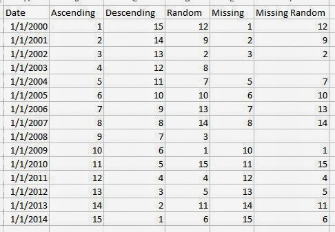
First, we have a complete data set with years ranging from 2000 to 2014.  We also have five different numeric fields.  The first is ordered the same as the years.  The second is ordered in reversed/descending order.  The third is simply random.  The fourth is the same as the first, but with the years 2003 and 2008 missing.  The fifth is the same as the random one, but with the years 2003 and 2008 missing.  Now, let's start by passing ascending data and seeing if we get it back in the same order.

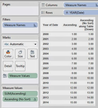
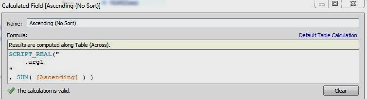
Ascending (No Sort)

Ascending (No Sort) by Year

As expected, R returned the data back exactly like it should have.  Now, let's try it with the random data to see if the values matter (they shouldn't).

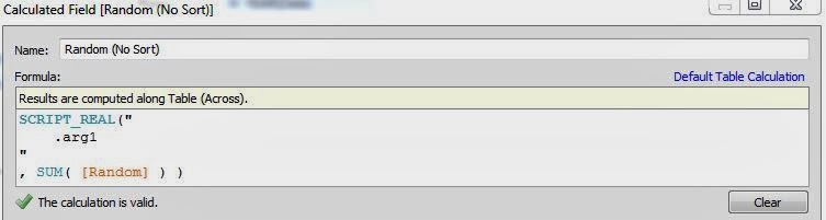
Random (No Sort)

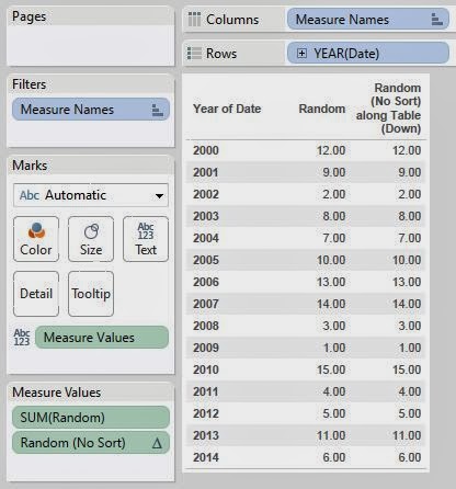
Random (No Sort) by Year

Again, no issues.  Finally, let's see if the missing values cause any problems.

Missing (No Sort)

Missing (No Sort) by Year

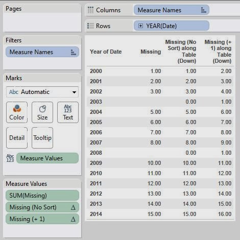
We finally have an interesting result.  Apparently, the SCRIPT_REAL function can't return NULL values.  R refers to these null values as NA.  This leads us to an interesting dilemma.  Is Tableau passing a Null and receiving a 0, or is Tableau passing a 0 initially.  We can test this.  First, let's show a simple example.

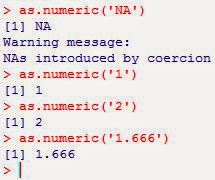
NA + 1

This picture shows that R is just like most languages in that you can't perform arithmetic on Null values.  So, let's use this to test what value R is receiving.

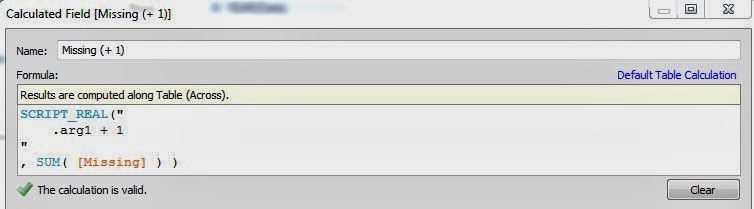
Missing (+ 1)

If R is receiving NAs, then this function should return NA, which Tableau would read as 0.  However, if Tableau is passing 0, then this function should return 1.  Let's see what happens.

Missing (+ 1) by Year

We see that Tableau is in fact passing 0 instead of Null.  This seems awkward to us.  Before we jump to any conclusions, let's confirm using a different method.

is.na

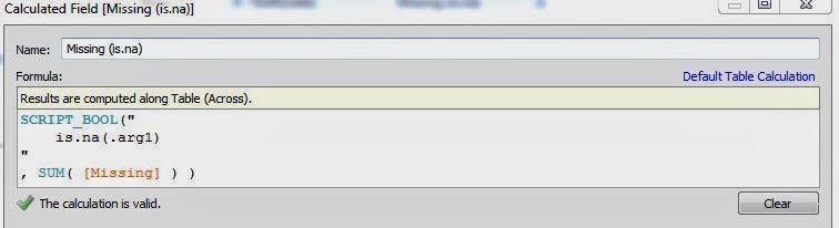
R has this nifty function called is.na() that returns true if the value is null.  So, let's run this test using Tableau.

Missing (is.na)

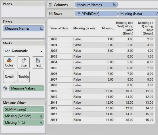
Missing (is.na) by Year

We have confirmed that Tableau is not passing Null values to R.  We don't see any reason why Tableau couldn't just pass NA in place of the Nulls.  Perhaps it has something to do with Rserve?  If you know anything, please let us know in the comments.  This leads us to another issue.  How do we combat this?  We have an idea, but let's see how R handles it.

Coercing NA

This is great!  It seems that if we pass the values to R as strings, then anything that isn't a number should be turned into NA.  This leads us to another question.  What does Tableau pass in place of a Null for Strings?

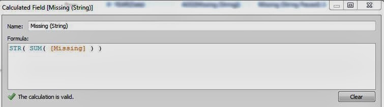
Missing (String)

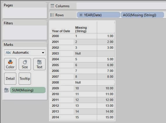
Missing (String) by Year

We see that Tableau coerces Null values into the string value "Null".  This is great.  Now, let's see what happens when pass it to R and coerce it back to a number.

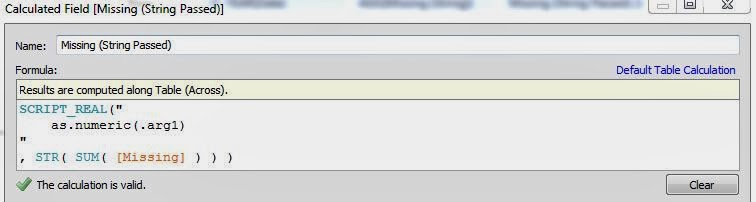
Missing (String Passed)

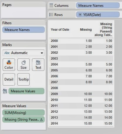
Missing (String Passed) by Year

Success!  We now know that if you have missing data, you can fix the problem by coercing them to strings before you pass them to R, then coercing them back to numbers in R.  However, this is a VERY serious issue.  It's shocking to us that a tool like Tableau would lack such simple functionality as Null handling.  We've put a post out of the Tableau forums to see if other people see it the same way.  You can see the post here.

EDIT:  Apparently this issue has been fixed in Tableau 8.1.3.

Now, let's move on to ordering.  What would happen if we passed the descending values to R, then sorted them and passed them back to Tableau?

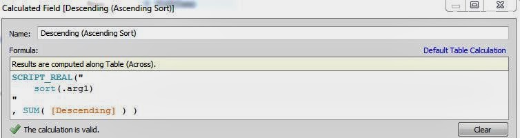
Descending (Ascending Sort)

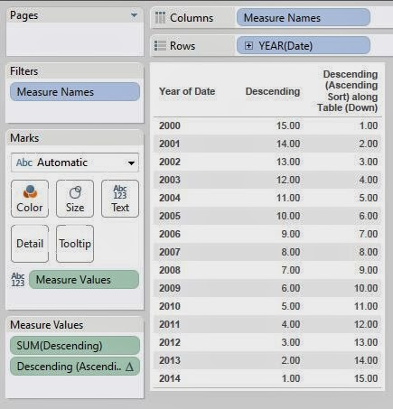
Descending (Ascending Sort) by Year

As you can see, Tableau was completely unaware that the data was sorted and sent it back in the order it was received.  This is a scary, yet unsurprising, result.  There are ways to handle this though.  Let's propose a real scenario for this.  Imagine that you want to create a time series that predicts the next value.  As we've seen in the last few posts, the data must be ordered in ascending order if you want to create a time series.  So, what would happen if we tried to pass in an unordered time series?

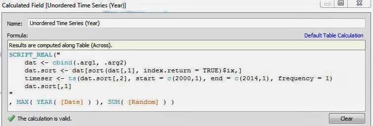
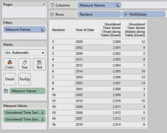
Unordered Time Series (Year)

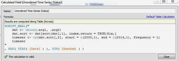
Unordered Time Series (Value)

Unordered Time Series (Table)

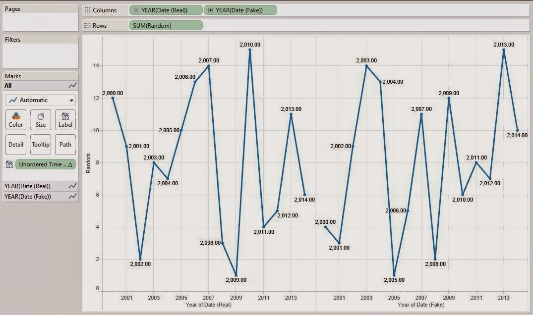
As you can see, the time series gets returned in ascending order, regardless of the order in which it was received.  You might ask "Who would look at a time series out of order like you have in this table?"  That's where the interesting idea comes in.  Consider the traditional way you would look at time series data.

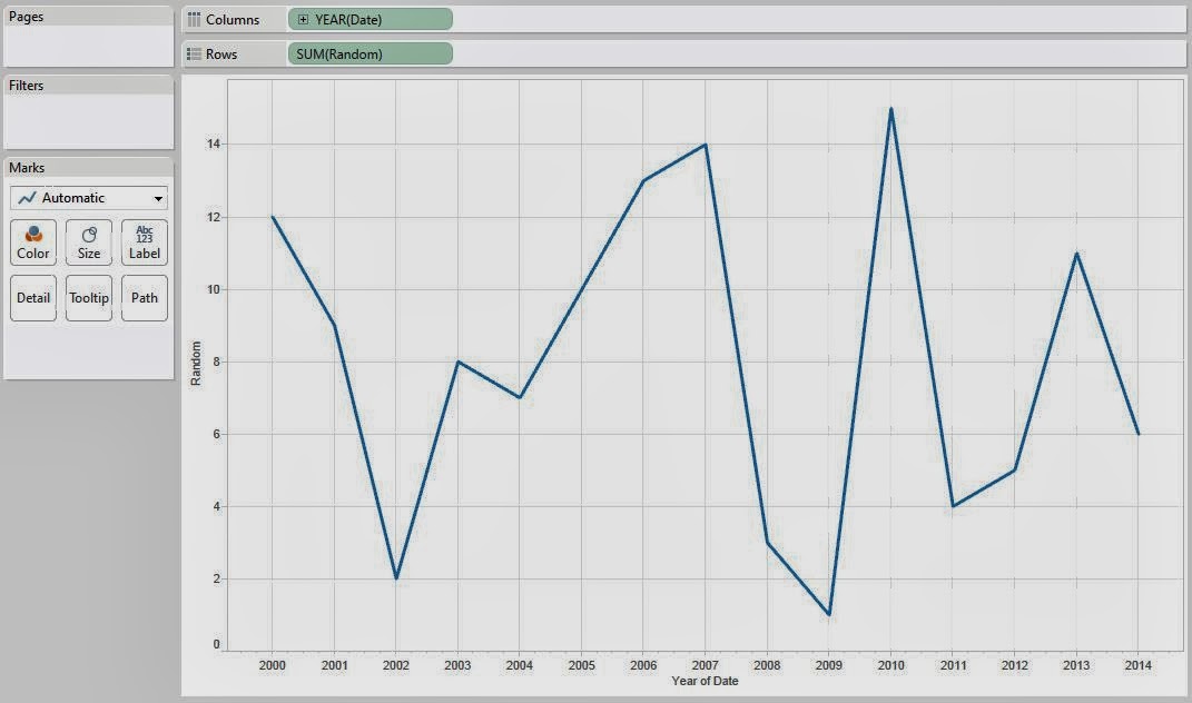
Time Series (Ordered)

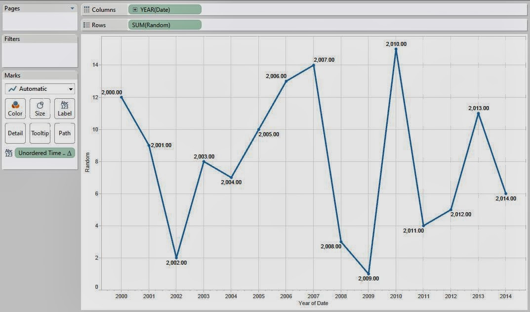
How do you know what order the data is in?  Can you assume that the data is in ascending order?  Well, if we overlay Unordered Time Series (Year), we will see if any of the years don't match up.

Time Series (Ordered) with Labels

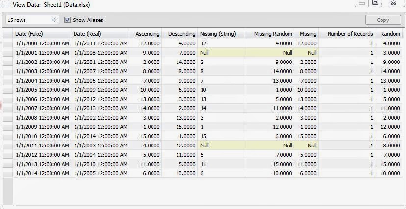
Following the labels, we see that everything is in order.  Is this always the case?  Our data was originally in ascending order by Year.  What if we were to reorder it?  When Tableau creates an extract, it automatically sorts the data.  We're not sure of the precise algorithm, but we do know that it was sorting our data by date.  So, we added another date in a different order in an attempt to trick Tableau into ordering the data improperly.

Data (Disordered)

Now, will our line chart still be in the correct order?

Time Series (Attempted Disordered)

As you can see, it doesn't matter whether the data is ordered or not.  These line charts always seem to be ordered by Date.  This is a very good thing.  It adds robustness to our procedures.  Now that we know these charts are always ordered, we can actually prevent a possible catastrophe.

Null Sorted

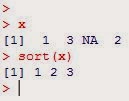
Notice how the NA gets removed when we sort?  If we were to sort data in R when we had missing data, we would be removing our missing data, which would have huge repercussions.  Namely, you can pass ten values to R and receive nine in return.  Tableau will toss an error if this happens.  Fortunately, this isn't a problem for our situations.  However, keep this in mind if you do find yourself in a situation where you are sorting data that may be missing.

In short, Tableau expects to receive data in the order in which it passes it.  Therefore, if you need to order your data, order it in Tableau BEFORE you pass it to R.  Tableau also doesn't pass Null numeric values to R, it passes zeros.  If you want to pass numeric data that may be missing, you may need to coerce the data to strings first.  Thanks for reading.  We hope you found this informative.

P.S.  Zen Master Jonathan Drummey has done a similar analysis and it can be found here.

Brad Llewellyn
Data Analytics Consultant
Mariner, LLC
llewellyn.wb@gmail.com
https://www.linkedin.com/in/bradllewellyn

Predictive Analytics in Tableau Part 10: Seasonal Decomposition

Today, we will talk about performing Seasonal Decomposition using Tableau 8.1's new R functionality.  Seasonal Decomposition is the process by which you determine what patterns over time exist in your data.  As usual, we will be using the Superstore Sales sample data set from Tableau.

Let's start by looking at our data.

Sales by Month

We can see that there is a definite "up-and-down" motion to the data.  This motion is known as "seasonality".  There also seems to be a very subtle downward trend to the data.  However, all of this relies on our eyes.  Let's use R to give us an actual decomposition.  It's important to note that this technique isn't necessarily used for prediction.  Therefore, the code is somewhat simplified because we won't be holding back observations.  Here's the code for Sales (Trend):

SCRIPT_REAL("
    library(forecast)

    year <- .arg1
    month <- .arg2
    sales <- .arg3
    len <- length(sales)

    ## Sorting the Data

    date <- year + month / 12
    dat <- cbind(year, month, sales)[sort(date, index.return = TRUE)$ix,]

    ## Decomposing the Time Series

    timeser <- ts(dat[,3], start = c(dat[1,1], dat[1,2]), end = c(dat[len,1], dat[len,2]), frequency = 12)
    as.vector(stl(timeser, s.window = 'period')[[1]][,2])
",

ATTR( YEAR( [Order Date] ) ), ATTR( MONTH( [Order Date] ) ), SUM( [Sales] ) )

Now, let's see what it looks like.

Sales by Month (with Tableau and R Trends)

On this chart, we chose to add Tableau's "Trend Line" as well for comparison.  What Tableau calls a "Trend Line" is actually a Regression line, which we saw quite a bit of in the first few posts of this series.  R's seasonal decomposition trend is an entirely different type of trend.  As you can see, the season decomposition trend adds much more information that the "Trend Line" does.  For any time series model, you don't want to consider the very early observations because they are based off of only a few observations.  So, let's filter out the year 2009 using a lookup (this way it doesn't affect our R calculations) so that we can really see what's going on.

Sales by Month (with Tableau and R Trends) (without 2009)

Now, we can see that Tableau's "Trend Line" seems to imply that sales are increasing.  However, the seasonal decomposition trend shows that it's more of a subtle wave than an increasing line.  In cases of time series data, the Regression-based "Trend Line" that Tableau uses could lead to some faulty assessments.  To be fair to Tableau, this "Trend Line" is perfect for scatterplots.

Sales by Quantity (with Trend)

Now that we've seen the overall trend, let's look at the seasonality.  As usual, the code is identical except for the last line.  The rest of the code can be found in the appendix at the end of the post.

as.vector(stl(timeser, s.window = 'period')[[1]][,1])

Let's see what it looks like.

Sales by Month (with Seasonality)

We see that the bottom chart repeats every year.  So, we can use this to say that our sales peak in late autumn and winter (September - January).  Strangely enough, our sales are average in November.  Perhaps there's some driving factor to this.  Maybe people are saving up money in November to buy Christmas presents in December.  Alas, we digress.  We can also see that sales are low in late spring and summer (April - August).  This is hugely impactful information that you might not have been able to determine using other methods.  On another note, imagine that we ran a huge sale in November 2011.  How do we tell if the sale gave us higher than expected returns?  Seasonal Decomposition can help here too.  Here the last line of code for Sales (Remainder)

as.vector(stl(timeser, s.window = 'period')[[1]][,3])

Sales by Month (with Remainder)

This chart shows us what was left once the Trend and Seasonality were removed, in other words, the remainder.  So, we see that November 2011 had sales significantly higher than expected.  Can this be explained by the sale we were running?  It's certainly seems so.  Of course, our analysis wouldn't end here if we were actually analyzing this.  Alas, this is just a demonstration.

Finally, let's look at a way to predict new observations using seasonal decomposition.  With seasonal decomposition, our predictions would always be equal to the trend plus the seasonal effect.  For new observations, we will always have the seasonal effect because it repeats every year.  However, we won't have the trend.  There are plenty of different methods you could come up with to determine the trend.  For this method, we'll just say that the trend for new observations is equal to the last trend we know (December 2012).  So, once we add a few blank lines to our data set (which we've done before to create new observations), we can create our calculation.  Here are the last few lines:

    seasdec <- stl(timeser, s.window = 'period')
    for(i in 1:len.new){if(dat.new[i,2] == month.orig[len.new + 1]){start <- i; break;}}
    pred <- seasdec[[1]][start:(start + hold.orig[1] - 1),1] + seasdec[[1]][len.new,2]
    c(rep(NA,len.new),pred)

Let's see what it looks like.

Sales by Month (With Forecast)

We can see that the forecasting process seems to be working.  It spikes in January and falls towards the middle of the year, which is what we expected.  In fairness, we're convinced that the usefulness of this procedure is in the analysis using remainders and seasonality, not in the forecasting.  Hopefully, this piqued your interest to give it a whirl.  Thanks for reading.  We hope you found this informative.

Brad Llewellyn
Data Analytics Consultant
Mariner, LLC
llewellyn.wb@gmail.com
https://www.linkedin.com/in/bradllewellyn

Appendix

Sales (Trend)

SCRIPT_REAL("
    library(forecast)

    year <- .arg1
    month <- .arg2
    sales <- .arg3
    len <- length(sales)

    ## Sorting the Data

    date <- year + month / 12
    dat <- cbind(year, month, sales)[sort(date, index.return = TRUE)$ix,]

    ## Decomposing the Time Series

    timeser <- ts(dat[,3], start = c(dat[1,1], dat[1,2]), end = c(dat[len,1], dat[len,2]), frequency = 12)
    as.vector(stl(timeser, s.window = 'period')[[1]][,2])
",


ATTR( YEAR( [Order Date] ) ), ATTR( MONTH( [Order Date] ) ), SUM( [Sales] ) )

Sales (Seasonality)

SCRIPT_REAL("
    library(forecast)

    year <- .arg1
    month <- .arg2
    sales <- .arg3
    len <- length(sales)

    ## Sorting the Data

    date <- year + month / 12
    dat <- cbind(year, month, sales)[sort(date, index.return = TRUE)$ix,]

    ## Decomposing the Time Series

    timeser <- ts(dat[,3], start = c(dat[1,1], dat[1,2]), end = c(dat[len,1], dat[len,2]), frequency = 12)
    as.vector(stl(timeser, s.window = 'period')[[1]][,1])
",


ATTR( YEAR( [Order Date] ) ), ATTR( MONTH( [Order Date] ) ), SUM( [Sales] ) )

Sales (Remainder)

SCRIPT_REAL("
    library(forecast)

    year <- .arg1
    month <- .arg2
    sales <- .arg3
    len <- length(sales)

    ## Sorting the Data

    date <- year + month / 12
    dat <- cbind(year, month, sales)[sort(date, index.return = TRUE)$ix,]

    ## Decomposing the Time Series

    timeser <- ts(dat[,3], start = c(dat[1,1], dat[1,2]), end = c(dat[len,1], dat[len,2]), frequency = 12)
    as.vector(stl(timeser, s.window = 'period')[[1]][,3])
",


ATTR( YEAR( [Order Date] ) ), ATTR( MONTH( [Order Date] ) ), SUM( [Sales] ) )

Sales (Forecast)

SCRIPT_REAL("
    library(forecast)

## Creating vectors

    hold.orig <- .arg4
    len.orig <- length( hold.orig )
    len.new <- len.orig - hold.orig[1]

    year.orig <- .arg1
    month.orig <- .arg2
    sales.orig <- .arg3

    ## Sorting the Data

    date.orig <- year.orig + month.orig / 12
    dat.orig <- cbind(year.orig, month.orig, sales.orig)[sort(date.orig, index.return = TRUE)$ix,]
    dat.new <- dat.orig[1:len.new,]

    ## Decomposing the Time Series

    timeser <- ts(dat.new[,3], start = c(dat.new[1,1], dat.new[1,2]), end = c(dat.new[len.new,1], dat.new[len.new,2]), frequency = 12)
    seasdec <- stl(timeser, s.window = 'period')

    ## Predicting the new Observations

    for(i in 1:len.new){if(dat.new[i,2] == month.orig[len.new + 1]){start <- i; break;}}
    pred <- seasdec[[1]][start:(start + hold.orig[1] - 1),1] + seasdec[[1]][len.new,2]
    c(rep(NA,len.new),pred)
",


ATTR( YEAR( [Order Date] ) ), ATTR( MONTH( [Order Date] ) ), SUM( [Sales] ), [Months to Forecast] )

Predictive Analytics in Tableau Part 9: Automatic Time Series Analysis

Today, we will talk about automatically performing time series analysis using Tableau 8.1's new R functionality.  Up to now, we've looked at ways to determine which type of exponential or ARIMA model fits the data best.  However, the number of models can be overwhelming to an analyst with less statistical exposure.  Today, we'll look at how to let R choose the model for you.  As usual, we will use the Superstore Sales sample data set in Tableau.

Let's imagine that we came up with a candidate list of models and want to see which ones are better for our type of data.

Too Many models

Here, we can see that charts can easily get very messy to see which models are best when there are a lot of models.  So, what better way is there?  Now, we're going to introduce two functions that will help.  The function ets() will create an appropriate Exponential model for your data and auto.arima() will create an appropriate ARIMA model for your data.  Like always, the code is identical until the last couple of lines.  You can find the full code in the appendix at the end of this post.  Here are the last couple of lines:

Exponential Model

fit <- ets(timeser)

c(rep(NA, len.new), forecast(fit)[[4]][1:hold.orig])

ARIMA Model

fit <- auto.arima(timeser)
(rep(NA, len.new), forecast(fit)[[4]][1:hold.orig])

Now, let's look at our chart.

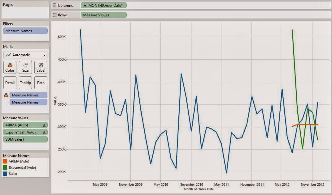
Automatic Models

As you can see, these calculations quickly gave us two "good" candidate models to look at.  You might notice that neither of these models fits the data extremely well.  However, we could look at these models and see that the ARIMA model doesn't seem to be able to account for any of the variability, which is a very bad thing.  The Exponential model seems much better, but still needs some tweaking.  Therefore, we could throw out all of the ARIMA models and focus on creating a better Exponential model.  In just a couple of minutes, we were able to narrow our modeling down to a single family!  That's a huge time saver.  Perhaps we could even improve this process by adding new functions and new techniques.  But, that's a topic for another post.  Thanks for reading.  We hope you found this informative.

Brad Llewellyn
Data Analytics Consultant
Mariner, LLC
llewellyn.wb@gmail.com
https://www.linkedin.com/in/bradllewellyn

Appendix

ARIMA (Auto)

SCRIPT_REAL("
    library(forecast)

    ## Creating vectors

    hold.orig <- .arg4
    len.orig <- length( hold.orig )
    len.new <- len.orig - hold.orig[1]

    year.orig <- .arg1
    month.orig <- .arg2
    sales.orig <- .arg3

    ## Sorting the Data

    date.orig <- year.orig + month.orig / 12
    dat.orig <- cbind(year.orig, month.orig, sales.orig)[sort(date.orig, index.return = TRUE)$ix,]
    dat.new <- dat.orig[1:len.new,]

    ## Fitting the Time Series

    timeser <- ts(dat.new[,3], start = c(dat.new[1,1], dat.new[1,2]), end = c(dat.new[len.new,1], dat.new[len.new,2]), frequency = 12)
    fit <- auto.arima(timeser)
    c(rep(NA, len.new), forecast(fit)[[4]][1:hold.orig])
",


ATTR( MONTH( [Order Date] ) ), ATTR( YEAR( [Order Date] ) ), SUM( [Sales] ), [Months to Forecast] )

Exponential (Auto)

SCRIPT_REAL("
    library(forecast)

    ## Creating vectors

    hold.orig <- .arg4
    len.orig <- length( hold.orig )
    len.new <- len.orig - hold.orig[1]

    year.orig <- .arg1
    month.orig <- .arg2
    sales.orig <- .arg3

    ## Sorting the Data

    date.orig <- year.orig + month.orig / 12
    dat.orig <- cbind(year.orig, month.orig, sales.orig)[sort(date.orig, index.return = TRUE)$ix,]
    dat.new <- dat.orig[1:len.new,]

    ## Fitting the Time Series

    timeser <- ts(dat.new[,3], start = c(dat.new[1,1], dat.new[1,2]), end = c(dat.new[len.new,1], dat.new[len.new,2]), frequency = 12)
    fit <- ets(timeser)
    c(rep(NA, len.new), forecast(fit)[[4]][1:hold.orig])
",


ATTR( MONTH( [Order Date] ) ), ATTR( YEAR( [Order Date] ) ), SUM( [Sales] ), [Months to Forecast] )

Predictive Analytics in Tableau Part 8: ARIMA Time Series

Today, we will talk about creating ARIMA time series models using Tableau 8.1's new R functionality.  In layman's terms, an ARIMA model uses three different numeric parameters to make varying types of time series models.  The ARIMA family is one of the most researched and respected families in the field of Time Series Analysis.  It is also used by a number of automated prediction tools like SQL Server Analysis Services.  As usual, we will use the Superstore Sales sample data set from Tableau.

The most important part of creating an ARIMA model is choosing the parameters.  The parameters are as follows:

AR  - Autoregressive
I      - Integrated
MA - Moving Average

We won't delve heavily into what each of these parameters does.  However, we will talk about methods for selecting them.  First, let's take a look at our data.

Sales by Month

Now, let's look at choosing the AR parameter.  In order to do this, we need to look at the Partial Autocorrelation Function (PACF).  Just like with the previous posts, almost all of the code is used to create the time series.  Only the last line is used to give us the PACF values.  The full code can be found in the appendix at the end of the post.

rep(pacf(timeser, plot=FALSE)$acf,5)[1:len.orig]

Now, let's look at these values.

Sales by Month (PACF)

The question we want to ask is "Starting at the beginning, how many consecutive values are above .25 or below -.25?"  We can easily accomplish this with colors.

AR Colors

Sales by Month (PACF with Color)

We can see that there are no values above .25 or below -.25.  So, there doesn't seem to be an AR component to this model.  Next, let's move on to the MA component using a very similar technique.  Moving Average components can be analyzed using the Autocorrelation Function (ACF).  Here's the last line of code.

rep(acf(timeser, plot=FALSE)$acf,5)[1:len.orig]

Now, let's look at the values.

Sales by Month (ACF with Color)

The first value is always guaranteed to be 1 and should be ignored.  We see that the values after one aren't really worth noting.  Therefore, the MA component in the model is 0 and the AR component is 0.  Now, let's look at the Integrated portion of the model.  R has a nice built-in function called ndiffs() that tells us what the I component should be.  Here's the last line of code.

ndiffs(timeser)

Now, let's see the value.

Sales by Month (I Component)

Here, we see that our I component should be zero.  This leaves us with a bit of an interesting conundrum.  An ARIMA(0,0,0) model is basically useless.  It is guaranteed always return the mean (average) value.  So, this means that the ARIMA family is not a good fit for this data.  Just for kicks, let's swap this data out for another data set that does fall in the ARIMA family.  So, let's look at a data set with monthly Unemployment values for the US.

Unemployment by Month

Now, let's look at the ARIMA components.

Unemployment by Month (ARIMA Components)

We can see that there are 3 consecutive AR values above .25 or below -.25, and I of 0, and 2 MA values (the first of which we ignore).  So, our model should be ARIMA(3,0,1).  Now, let's see what our forecasts look like.

Unemployment by Month (Forecast)

We can see that the ARIMA model seems to be pretty good at predicting the up-and-down motion of the data.  However, the recent rise in unemployment has caused some variability that the model doesn't handle very well.  Fortunately, there are plenty of other families of models out there.  Thanks for reading.  We hope you found this informative.

Brad Llewellyn
Data Analytics Consultant
Mariner, LLC
llewellyn.wb@gmail.com
https://www.linkedin.com/in/bradllewellyn

EDIT: An anonymous user noted an error in the original appendix.  The R variables were defined as 

year.orig <- .arg1
month.orig <- .arg2

while our assignment at the end of the segment was defining

ATTR( MONTH( [Order Date] ) ) = .arg1
ATTR( YEAR( [Order Date] ) ) = .arg2

This has now been fixed an all of the code should be valid.  Many thanks to our readers for pointing that out.

Appendix

AR Component

SCRIPT_REAL("
    library(forecast)

    ## Creating vectors

    hold.orig <- .arg4
    len.orig <- length( hold.orig )
    len.new <- len.orig - hold.orig[1]

    year.orig <- .arg2
    month.orig <- .arg1
    sales.orig <- .arg3

    ## Sorting the Data

    date.orig <- year.orig + month.orig / 12
    dat.orig <- cbind(year.orig, month.orig, sales.orig)[sort(date.orig, index.return = TRUE)$ix,]
    dat.new <- dat.orig[1:len.new,]

    ## Fitting the Time Series

    timeser <- ts(dat.new[,3], start = c(dat.new[1,1], dat.new[1,2]), end = c(dat.new[len.new,1], dat.new[len.new,2]), frequency = 12)
    rep(pacf(timeser, plot=FALSE)$acf,5)[1:len.orig]
",

ATTR( MONTH( [Order Date] ) ), ATTR( YEAR( [Order Date] ) ), SUM( [Sales] ), [Months to Forecast] )

I Component

SCRIPT_REAL("
    library(forecast)

    ## Creating vectors

    hold.orig <- .arg4
    len.orig <- length( hold.orig )
    len.new <- len.orig - hold.orig[1]

    year.orig <- .arg2
    month.orig <- .arg1
    sales.orig <- .arg3

    ## Sorting the Data

    date.orig <- year.orig + month.orig / 12
    dat.orig <- cbind(year.orig, month.orig, sales.orig)[sort(date.orig, index.return = TRUE)$ix,]
    dat.new <- dat.orig[1:len.new,]

    ## Fitting the Time Series

    timeser <- ts(dat.new[,3], start = c(dat.new[1,1], dat.new[1,2]), end = c(dat.new[len.new,1], dat.new[len.new,2]), frequency = 12)
    ndiffs(timeser)
",

ATTR( MONTH( [Order Date] ) ), ATTR( YEAR( [Order Date] ) ), SUM( [Sales] ), [Months to Forecast] )

MA Component

SCRIPT_REAL("
    library(forecast)

    ## Creating vectors

    hold.orig <- .arg4
    len.orig <- length( hold.orig )
    len.new <- len.orig - hold.orig[1]

    year.orig <- .arg2
    month.orig <- .arg1
    sales.orig <- .arg3

    ## Sorting the Data

    date.orig <- year.orig + month.orig / 12
    dat.orig <- cbind(year.orig, month.orig, sales.orig)[sort(date.orig, index.return = TRUE)$ix,]
    dat.new <- dat.orig[1:len.new,]

    ## Fitting the Time Series

    timeser <- ts(dat.new[,3], start = c(dat.new[1,1], dat.new[1,2]), end = c(dat.new[len.new,1], dat.new[len.new,2]), frequency = 12)
    rep(acf(timeser, plot=FALSE)$acf,5)[1:len.orig]
",

ATTR( MONTH( [Order Date] ) ), ATTR( YEAR( [Order Date] ) ), SUM( [Sales] ), [Months to Forecast] )

Forecast (ARIMA(0,0,1))

SCRIPT_REAL("
    library(forecast)

    ## Creating vectors

    hold.orig <- .arg4
    len.orig <- length( hold.orig )
    len.new <- len.orig - hold.orig[1]

    year.orig <- .arg2
    month.orig <- .arg1
    sales.orig <- .arg3

    ## Sorting the Data

    date.orig <- year.orig + month.orig / 12
    dat.orig <- cbind(year.orig, month.orig, sales.orig)[sort(date.orig, index.return = TRUE)$ix,]
    dat.new <- dat.orig[1:len.new,]

    ## Fitting the Time Series

    timeser <- ts(dat.new[,3], start = c(dat.new[1,1], dat.new[1,2]), end = c(dat.new[len.new,1], dat.new[len.new,2]), frequency = 12)
    fit <- arima(timeser, order=c(0, 0, 0))
    c(rep(NA, len.new), forecast(fit)[[4]][1:hold.orig])
",

ATTR( MONTH( [Order Date] ) ), ATTR( YEAR( [Order Date] ) ), SUM( [Sales] ), [Months to Forecast] )

Forecast (ARIMA(3,0,1))

SCRIPT_REAL("
    library(forecast)

    ## Creating vectors

    hold.orig <- .arg4
    len.orig <- length( hold.orig )
    len.new <- len.orig - hold.orig[1]

    year.orig <- .arg2
    month.orig <- .arg1
    sales.orig <- .arg3

    ## Sorting the Data

    date.orig <- year.orig + month.orig / 12
    dat.orig <- cbind(year.orig, month.orig, sales.orig)[sort(date.orig, index.return = TRUE)$ix,]
    dat.new <- dat.orig[1:len.new,]

    ## Fitting the Time Series

    timeser <- ts(dat.new[,3], start = c(dat.new[1,1], dat.new[1,2]), end = c(dat.new[len.new,1], dat.new[len.new,2]), frequency = 12)
    fit <- arima(timeser, order=c(3, 0, 1))
    c(rep(NA, len.new), forecast(fit)[[4]][1:hold.orig])
",

ATTR( MONTH( [Order Date] ) ), ATTR( YEAR( [Order Date] ) ), SUM( [Sales] ), [Months to Forecast] )

Predictive Analytics in Tableau Part 7: Double and Triple Exponential Time Series

Today, we will talk about creating Double and Triple Exponential Time Series using Tableau 8.1's new R functionality.  If you read our previous post, Single Exponential Time Series, you remember that we were only able to predict a constant value for all future observations.  Trend and Seasonality were not considered using the Single Exponential.  These models should fix all of that.  Once again, we will use the Superstore Sales sample data set from Tableau.

At its core, a single exponential time series can predict values without trend (increase or decrease over longer periods of time) or seasonality (repetition of patterns at regular intervals, i.e. yearly, monthly, etc.).  The double exponential time series adds trend to the model while the triple exponential time series adds trend and seasonality.  We're also adding the model that accounts for seasonality without accounting for trend.  We're not sure what this model is called, so we'll call it the Reverse Double Exponential Model for now.  If you have any idea what it's called or if it's invalid for some reason, please let us know in the comments.  The code is almost identical like before, just with the second to last line changed.  You can find the full code in the appendix at the end of this post.

Double Exponential

fit <- HoltWinters(timeser, gamma=FALSE)

Reverse Double Exponential

fit <- HoltWinters(timeser, beta=FALSE)

Triple Exponential

fit <- HoltWinters(timeser)

Now, let's look at these predictions.

Sales by Month (Predictions)

We can see that the green line (Double Exponential) is straight.  This is exactly what we expected.  However, there is some definite seasonality in this data that we need to account for.  The orange line (Triple Exponential) seems to follow that seasonality, but the trend seems to have pushed it too high.  The red line (Reverse Double Exponential) appears to be the "Goldilocks" model.  It accounts for the seasonality, but doesn't let the trend drag it too high.  For further examination, let's look at the 95% confidence intervals for these models to see which models fit the data more tightly.

Sales by Month (Bounds)

We can easily see that the green bounds (Double Exponential) are so spread out that they become basically worthless.  Also, the orange bounds (Triple Exponential) and the red bounds (Reverse Double Exponential) seem to the same except that the orange bounds are shifted up slightly higher, which is exactly what we saw with the predictions as well.  Therefore, we have good evidence to say that the Reverse Double Exponential model is the best fit for this data.  Now, let's use the same trick as last week to predict new values by adding blank rows to our data set.

Sales by Month (Reverse Double Exponential with Bounds)

Now, we have seemingly accurate predictions using a well-respected time series model.  However, we're not done with this yet.  There are other families of time series models we could use.  There's also artificial neural networks, naive bayes, and much more.  Thanks for reading.  We hope you found this informative.

Brad Llewellyn
Data Analytics Consultant
Mariner, LLC
llewellyn.wb@gmail.com
https://www.linkedin.com/in/bradllewellyn

Appendix

Double Exponential

SCRIPT_REAL("
    library(forecast)

    ## Creating vectors

    hold.orig <- .arg4
    len.orig <- length( hold.orig )
    len.new <- len.orig - hold.orig[1]

    year.orig <- .arg1
    month.orig <- .arg2
    sales.orig <- .arg3

    ## Sorting the Data

    date.orig <- year.orig + month.orig / 12
    dat.orig <- cbind(year.orig, month.orig, sales.orig)[sort(date.orig, index.return = TRUE)$ix,]
    dat.new <- dat.orig[1:len.new,]

    ## Fitting the Time Series

    timeser <- ts(dat.new[,3], start = c(dat.new[1,1], dat.new[1,2]), end = c(dat.new[len.new,1], dat.new[len.new,2]), frequency = 12)
    fit <- HoltWinters(timeser, gamma=FALSE)
    c(rep(NA,len.new), forecast(fit, hold.orig[1])$mean)
"
, ATTR( YEAR( [Order Date] ) ), ATTR( MONTH( [Order Date] ) ), SUM( [Sales] ),
 [Months to Forecast] )

Double Exponential (Lower 95%)

SCRIPT_REAL("
    library(forecast)

    ## Creating vectors

    hold.orig <- .arg4
    len.orig <- length( hold.orig )
    len.new <- len.orig - hold.orig[1]

    year.orig <- .arg1
    month.orig <- .arg2
    sales.orig <- .arg3

    ## Sorting the Data

    date.orig <- year.orig + month.orig / 12
    dat.orig <- cbind(year.orig, month.orig, sales.orig)[sort(date.orig, index.return = TRUE)$ix,]
    dat.new <- dat.orig[1:len.new,]

    ## Fitting the Time Series

    timeser <- ts(dat.new[,3], start = c(dat.new[1,1], dat.new[1,2]), end = c(dat.new[len.new,1], dat.new[len.new,2]), frequency = 12)
    fit <- HoltWinters(timeser, gamma=FALSE)
    c(rep(NA,len.new), forecast(fit, hold.orig[1])$lower[,2])
"
, ATTR( YEAR( [Order Date] ) ), ATTR( MONTH( [Order Date] ) ), SUM( [Sales] ),

 [Months to Forecast] )

Double Exponential (Upper 95%)

SCRIPT_REAL("
    library(forecast)

    ## Creating vectors

    hold.orig <- .arg4
    len.orig <- length( hold.orig )
    len.new <- len.orig - hold.orig[1]

    year.orig <- .arg1
    month.orig <- .arg2
    sales.orig <- .arg3

    ## Sorting the Data

    date.orig <- year.orig + month.orig / 12
    dat.orig <- cbind(year.orig, month.orig, sales.orig)[sort(date.orig, index.return = TRUE)$ix,]
    dat.new <- dat.orig[1:len.new,]

    ## Fitting the Time Series

    timeser <- ts(dat.new[,3], start = c(dat.new[1,1], dat.new[1,2]), end = c(dat.new[len.new,1], dat.new[len.new,2]), frequency = 12)
    fit <- HoltWinters(timeser, gamma=FALSE)
    c(rep(NA,len.new), forecast(fit, hold.orig[1])$upper[,2])
"
, ATTR( YEAR( [Order Date] ) ), ATTR( MONTH( [Order Date] ) ), SUM( [Sales] ),

 [Months to Forecast] )

Reverse Double Exponential

SCRIPT_REAL("
    library(forecast)

    ## Creating vectors

    hold.orig <- .arg4
    len.orig <- length( hold.orig )
    len.new <- len.orig - hold.orig[1]

    year.orig <- .arg1
    month.orig <- .arg2
    sales.orig <- .arg3

    ## Sorting the Data

    date.orig <- year.orig + month.orig / 12
    dat.orig <- cbind(year.orig, month.orig, sales.orig)[sort(date.orig, index.return = TRUE)$ix,]
    dat.new <- dat.orig[1:len.new,]

    ## Fitting the Time Series

    timeser <- ts(dat.new[,3], start = c(dat.new[1,1], dat.new[1,2]), end = c(dat.new[len.new,1], dat.new[len.new,2]), frequency = 12)
    fit <- HoltWinters(timeser, beta=FALSE)
    c(rep(NA,len.new), forecast(fit, hold.orig[1])$mean)
"
, ATTR( YEAR( [Order Date] ) ), ATTR( MONTH( [Order Date] ) ), SUM( [Sales] ),
 [Months to Forecast] )

Reverse Double Exponential (Lower 95%)

SCRIPT_REAL("
    library(forecast)

    ## Creating vectors

    hold.orig <- .arg4
    len.orig <- length( hold.orig )
    len.new <- len.orig - hold.orig[1]

    year.orig <- .arg1
    month.orig <- .arg2
    sales.orig <- .arg3

    ## Sorting the Data

    date.orig <- year.orig + month.orig / 12
    dat.orig <- cbind(year.orig, month.orig, sales.orig)[sort(date.orig, index.return = TRUE)$ix,]
    dat.new <- dat.orig[1:len.new,]

    ## Fitting the Time Series

    timeser <- ts(dat.new[,3], start = c(dat.new[1,1], dat.new[1,2]), end = c(dat.new[len.new,1], dat.new[len.new,2]), frequency = 12)
    fit <- HoltWinters(timeser, beta=FALSE)
    c(rep(NA,len.new), forecast(fit, hold.orig[1])$lower[,2])
"
, ATTR( YEAR( [Order Date] ) ), ATTR( MONTH( [Order Date] ) ), SUM( [Sales] ),

 [Months to Forecast] )

Reverse Double Exponential (Upper 95%)

SCRIPT_REAL("
    library(forecast)

    ## Creating vectors

    hold.orig <- .arg4
    len.orig <- length( hold.orig )
    len.new <- len.orig - hold.orig[1]

    year.orig <- .arg1
    month.orig <- .arg2
    sales.orig <- .arg3

    ## Sorting the Data

    date.orig <- year.orig + month.orig / 12
    dat.orig <- cbind(year.orig, month.orig, sales.orig)[sort(date.orig, index.return = TRUE)$ix,]
    dat.new <- dat.orig[1:len.new,]

    ## Fitting the Time Series

    timeser <- ts(dat.new[,3], start = c(dat.new[1,1], dat.new[1,2]), end = c(dat.new[len.new,1], dat.new[len.new,2]), frequency = 12)
    fit <- HoltWinters(timeser, beta=FALSE)
    c(rep(NA,len.new), forecast(fit, hold.orig[1])$upper[,2])
"
, ATTR( YEAR( [Order Date] ) ), ATTR( MONTH( [Order Date] ) ), SUM( [Sales] ),

 [Months to Forecast] )

Triple Exponential

SCRIPT_REAL("
    library(forecast)

    ## Creating vectors

    hold.orig <- .arg4
    len.orig <- length( hold.orig )
    len.new <- len.orig - hold.orig[1]

    year.orig <- .arg1
    month.orig <- .arg2
    sales.orig <- .arg3

    ## Sorting the Data

    date.orig <- year.orig + month.orig / 12
    dat.orig <- cbind(year.orig, month.orig, sales.orig)[sort(date.orig, index.return = TRUE)$ix,]
    dat.new <- dat.orig[1:len.new,]

    ## Fitting the Time Series

    timeser <- ts(dat.new[,3], start = c(dat.new[1,1], dat.new[1,2]), end = c(dat.new[len.new,1], dat.new[len.new,2]), frequency = 12)
    fit <- HoltWinters(timeser)
    c(rep(NA,len.new), forecast(fit, hold.orig[1])$mean)
"
, ATTR( YEAR( [Order Date] ) ), ATTR( MONTH( [Order Date] ) ), SUM( [Sales] ),

 [Months to Forecast] )

Triple Exponential (Lower 95%)

SCRIPT_REAL("
    library(forecast)

    ## Creating vectors

    hold.orig <- .arg4
    len.orig <- length( hold.orig )
    len.new <- len.orig - hold.orig[1]

    year.orig <- .arg1
    month.orig <- .arg2
    sales.orig <- .arg3

    ## Sorting the Data

    date.orig <- year.orig + month.orig / 12
    dat.orig <- cbind(year.orig, month.orig, sales.orig)[sort(date.orig, index.return = TRUE)$ix,]
    dat.new <- dat.orig[1:len.new,]

    ## Fitting the Time Series

    timeser <- ts(dat.new[,3], start = c(dat.new[1,1], dat.new[1,2]), end = c(dat.new[len.new,1], dat.new[len.new,2]), frequency = 12)
    fit <- HoltWinters(timeser)
    c(rep(NA,len.new), forecast(fit, hold.orig[1])$lower[,2])
"
, ATTR( YEAR( [Order Date] ) ), ATTR( MONTH( [Order Date] ) ), SUM( [Sales] ),

 [Months to Forecast] )

Triple Exponential (Upper 95%)

SCRIPT_REAL("
    library(forecast)

    ## Creating vectors

    hold.orig <- .arg4
    len.orig <- length( hold.orig )
    len.new <- len.orig - hold.orig[1]

    year.orig <- .arg1
    month.orig <- .arg2
    sales.orig <- .arg3

    ## Sorting the Data

    date.orig <- year.orig + month.orig / 12
    dat.orig <- cbind(year.orig, month.orig, sales.orig)[sort(date.orig, index.return = TRUE)$ix,]
    dat.new <- dat.orig[1:len.new,]

    ## Fitting the Time Series

    timeser <- ts(dat.new[,3], start = c(dat.new[1,1], dat.new[1,2]), end = c(dat.new[len.new,1], dat.new[len.new,2]), frequency = 12)
    fit <- HoltWinters(timeser)
    c(rep(NA,len.new), forecast(fit, hold.orig[1])$upper[,2])
"
, ATTR( YEAR( [Order Date] ) ), ATTR( MONTH( [Order Date] ) ), SUM( [Sales] ),

 [Months to Forecast] )

Predictive Analytics in Tableau Part 6: Single Exponential Time Series

Before we start today's topic, we want to direct you towards a great source of information about Tableau 8.1's R functionality.  This page was compiled by members of the Tableau community and can be found here.  Now, on to the demonstration.

Today, we will talk about creating time series analyses using Tableau 8.1's new R functionality.  In our previous demonstrations, we used varying regression techniques to predict values.  These techniques took into account the relationships between the variables, but not across time.  Time Series Analyses approach from the opposite direction.  They attempt to predict new values by looking at previous (or future) values in time, but only considering one variable.  For this demonstration, we will use the Superstore Sales sample data set from Tableau.

As always, the first step is to look at the data we want to forecast.  Let's look at Total Sales per Month.

Sales by Month

We can see that there is quite a bit of variation in this data.  Now, we run into our first conundrum.  I don't know of an easy way to allow Tableau to see dates outside of what's in the data.  Therefore, we can only forecast for dates we already have in the data.  This is actually a good and bad thing for us, as we'll soon see.  If you have a system that includes budget data for the future, then the dates will already be available and you won't have this problem.  Alas, we do not have such luck.  So, let's first hold out the last six months of our data and create the model using only data up to June 2012.  That way, we have something to compare our forecasts to.  In order to do this, we create an integer parameter.

Months to Forecast

Now, we can dynamically set the number of months we want to forecast.  Next, we need to create the code to do this.  But, before we do that, we need to install the "forecast" package on the R Server.

Install Packages

If you don't have the access to do this, then you will probably need to talk to the administrator on your R server.  Fortunately, we host the server on our local machine; so, there is no issue.  Now, back to the forecasting.

This code is long and somewhat complex.  So, we'll only touch on the important parts.  The code for Sales (Forecast) is as follows:

SCRIPT_REAL("
    library(forecast)

    ## Creating vectors

    hold.orig <- .arg4
    len.orig <- length( hold.orig )
    len.new <- len.orig - hold.orig[1]

    year.orig <- .arg1
    month.orig <- .arg2
    sales.orig <- .arg3

    ## Sorting the Data

    date.orig <- year.orig + month.orig / 12
    dat.orig <- cbind(year.orig, month.orig, sales.orig)[sort(date.orig, index.return = TRUE)$ix,]
    dat.new <- dat.orig[1:len.new,]

    ## Fitting the Time Series

    timeser <- ts(dat.new[,3], start = c(dat.new[1,1], dat.new[1,2]), end = c(dat.new[len.new,1],
                     dat.new[len.new,2]), frequency = 12)
    fit <- HoltWinters(timeser, beta=FALSE, gamma=FALSE)
    c(rep(NA,len.new), forecast(fit, hold.orig[1])$mean)
"
, ATTR( YEAR( [Order Date] ) ), ATTR( MONTH( [Order Date] ) ), SUM( [Sales] ),
 [Months to Forecast] )

First, we need to install the forecast library using library(forecast).  Then, we need to sort the data by date, and hold out the last few months.  How many months get held out depends on the value of our [Months to Forecast] parameter.  Finally, we fit our time series as a single exponential model and output the results.  Let's see what it looks like.

Sales by Month (with Forecast)

As you can see, the forecast is pretty close to the true values.  This type of model cannot pick up on the trend or seasonality though.  We'll deal with that in a later post.  For now, let's see how well this model fits by also plotting the 80% and 95% confidence intervals.  You should remember confidence intervals from our posts about regression.  The code for the intervals are identical to the code for the forecast, with the exception of the last line of code.  I'll post the final lines here.  If you want to see the full code, please refer to the appendix at the end of this post.

Sales (Forecast) (Lower 80%)

c(rep(NA,len.new), forecast(fit, hold.orig[1])$lower[,1])

Sales (Forecast) (Lower 95%)

c(rep(NA,len.new), forecast(fit, hold.orig[1])$lower[,2])

Sales (Forecast) (Upper 80%)

c(rep(NA,len.new), forecast(fit, hold.orig[1])$upper[,1])

Sales (Forecast) (Upper 95%)

c(rep(NA,len.new), forecast(fit, hold.orig[1])$upper[,2])

Now, let's see what the intervals look like

Sales by Month (with Forecast and Bounds)

We can see that all of the actual values fall well within the 95% bound.  This means that our model fits our data reasonably well.  Now, let's talk about how to use this model to predict future values.  The simplest way we could find to do this is to add some filler lines to your data set.  In our case, we're using an Excel spreadsheet.  So, we add the following lines to our data.

Adding Empty Dates

You should note that if you are doing forecasts for a specific type of product, customer, etc., you will need to duplicate these dates for every combination of dimensions you want to forecast over.  Now, when we refresh our worksheet, we have our forecasts.

Sales by Month (with Future Forecast and Bounds)

One very important thing to notice about these forecasts is that the bounds are extremely far from the graph.  This would seem to imply that the model is not a good fit for the data.  Therefore, we would want to use a different type of time series model for it.  Unfortunately, that's going to have to wait until the next post.  Thanks for reading.  We hope you found this informative.

P.S.

If anybody can think of a better way to get future forecasts for dates that don't exist in the data, please let us know in the comments.  Also, this method is not robust against missing data.  If you're data has some missing months/week/etc., you may have to alter the method slightly.

Brad Llewellyn
Data Analytics Consultant
Mariner, LLC
llewellyn.wb@gmail.com
https://www.linkedin.com/in/bradllewellyn

APPENDIX:

The code for Sales (Forecast) (Lower 80%) is as follows:

SCRIPT_REAL("
    library(forecast)

    ## Creating vectors

    hold.orig <- .arg4
    len.orig <- length( hold.orig )
    len.new <- len.orig - hold.orig[1]

    year.orig <- .arg1
    month.orig <- .arg2
    sales.orig <- .arg3

    ## Sorting the Data

    date.orig <- year.orig + month.orig / 12
    dat.orig <- cbind(year.orig, month.orig, sales.orig)[sort(date.orig, index.return = TRUE)$ix,]
    dat.new <- dat.orig[1:len.new,]

    ## Fitting the Time Series

    timeser <- ts(dat.new[,3], start = c(dat.new[1,1], dat.new[1,2]), end = c(dat.new[len.new,1], dat.new[len.new,2]), frequency = 12)
    fit <- HoltWinters(timeser, beta=FALSE, gamma=FALSE)
    c(rep(NA,len.new), forecast(fit, hold.orig[1])$lower[,1])
"
, ATTR( YEAR( [Order Date] ) ), ATTR( MONTH( [Order Date] ) ), SUM( [Sales] ),
 [Months to Forecast] )

The code for Sales (Forecast) (Lower 95%) is as follows:

SCRIPT_REAL("
    library(forecast)

    ## Creating vectors

    hold.orig <- .arg4
    len.orig <- length( hold.orig )
    len.new <- len.orig - hold.orig[1]

    year.orig <- .arg1
    month.orig <- .arg2
    sales.orig <- .arg3

    ## Sorting the Data

    date.orig <- year.orig + month.orig / 12
    dat.orig <- cbind(year.orig, month.orig, sales.orig)[sort(date.orig, index.return = TRUE)$ix,]
    dat.new <- dat.orig[1:len.new,]

    ## Fitting the Time Series

    timeser <- ts(dat.new[,3], start = c(dat.new[1,1], dat.new[1,2]), end = c(dat.new[len.new,1], dat.new[len.new,2]), frequency = 12)
    fit <- HoltWinters(timeser, beta=FALSE, gamma=FALSE)
    c(rep(NA,len.new), forecast(fit, hold.orig[1])$lower[,2])
"
, ATTR( YEAR( [Order Date] ) ), ATTR( MONTH( [Order Date] ) ), SUM( [Sales] ),

 [Months to Forecast] )

The code for Sales (Forecast) (Upper 80%) is as follows:

SCRIPT_REAL("
    library(forecast)

    ## Creating vectors

    hold.orig <- .arg4
    len.orig <- length( hold.orig )
    len.new <- len.orig - hold.orig[1]

    year.orig <- .arg1
    month.orig <- .arg2
    sales.orig <- .arg3

    ## Sorting the Data

    date.orig <- year.orig + month.orig / 12
    dat.orig <- cbind(year.orig, month.orig, sales.orig)[sort(date.orig, index.return = TRUE)$ix,]
    dat.new <- dat.orig[1:len.new,]

    ## Fitting the Time Series

    timeser <- ts(dat.new[,3], start = c(dat.new[1,1], dat.new[1,2]), end = c(dat.new[len.new,1], dat.new[len.new,2]), frequency = 12)
    fit <- HoltWinters(timeser, beta=FALSE, gamma=FALSE)
    c(rep(NA,len.new), forecast(fit, hold.orig[1])$upper[,1])
"
, ATTR( YEAR( [Order Date] ) ), ATTR( MONTH( [Order Date] ) ), SUM( [Sales] ),

 [Months to Forecast] )

The code for Sales (Forecast) (Upper 95%) is as follows:

SCRIPT_REAL("
    library(forecast)

    ## Creating vectors

    hold.orig <- .arg4
    len.orig <- length( hold.orig )
    len.new <- len.orig - hold.orig[1]

    year.orig <- .arg1
    month.orig <- .arg2
    sales.orig <- .arg3

    ## Sorting the Data

    date.orig <- year.orig + month.orig / 12
    dat.orig <- cbind(year.orig, month.orig, sales.orig)[sort(date.orig, index.return = TRUE)$ix,]
    dat.new <- dat.orig[1:len.new,]

    ## Fitting the Time Series

    timeser <- ts(dat.new[,3], start = c(dat.new[1,1], dat.new[1,2]), end = c(dat.new[len.new,1], dat.new[len.new,2]), frequency = 12)
    fit <- HoltWinters(timeser, beta=FALSE, gamma=FALSE)
    c(rep(NA,len.new), forecast(fit, hold.orig[1])$upper[,2])
"
, ATTR( YEAR( [Order Date] ) ), ATTR( MONTH( [Order Date] ) ), SUM( [Sales] ),

 [Months to Forecast] )