Introduction to Table Calculations: Compute Using

Today, we will talk about basic table calculations.  More specifically, we will talk about the Compute Using feature.  We believe that this is the most important, yet most undervalued, feature of table calculations.  In fact, almost all of the table calculation posts on the forums are handled with a simple use of Compute Using.  As usual, we will use the Superstore Sales sample data set in Tableau.

Step 1:

• Create a calculation that returns 1 for every cell
• Create the following calculated field

1

Step 2:

• Create a calculation that counts 1, 2, 3, etc. through the cells
• Create the following calculated field
• Duplicate this field a few times

Running Sum of 1

A more advanced user might recognize that this is what the INDEX() function is designed to do.  We agree entirely; but, we felt it was simpler to understand using a running sum, which most people should already know.

Step 3:

• Drag YEAR( [Order Date] ) onto the Rows Shelf.
• Drag 2 of the Running Sum fields onto the the chart as text.

Table (Down)

As you can see, the default direction is Table (Down).  This means that the table calculation will continue to move down the table until it reaches the end, never restarting.

Step 4:

• Change the Compute Using on one of the Running Sums to use Cell

Compute Using Cell

Cell

As you can see, Cell refers to the current row.  In fact, Table Calculations at the cell level are not very useful, except in extremely rare cases.

Step 5:

• Drag MONTH( [Order Date] ) onto the Rows Shelf as well.
• Add another copy of Running Sum to the chart, with Compute Using: Pane (Down)

Pane (Down)

Now, we can see that Table (Down) still runs the entire table and Cell runs nowhere.  The point to notice here is Pane (Down) restarts every year.  More specifically, the Pane is area between the table and the cell.  Here is a good illustration of the concept.

2 Dimension Illustration

Now, you might question something.  What happens if there are more than dimensions?  Which one is the Pane?  Let's take a look

Step 6:

• Add QUARTER( [Order Date] ) to the Rows Shelf between Year and Month

3 Dimensions

As you can see, the Pane restarts every Quarter, not every Year.  This means that the Pane is the area just larger than the Cell, regardless of the number of dimensions in the Table.  The following illustration should help.

3 Dimension Illustration

We don't know what to call the area(s) between the Table and the Pane.  If you want to work in this area, you will have to get more explicit with your Compute Using.  We will explain this in a later post.  Lastly, let's look at directions.

Step 7:

• Create a blank chart
• Place Year on the Rows Shelf
• Place Quarter on the Columns Shelf
• Place 4 copies of Running Sum on the chart as text
• Set each copy to use a different direction for Compute Using: Table, i.e (Down), (Across), etc.

Directions

As you can see, Table (Across) goes across the columns, then resets at every row.  Table (Down) does the opposite.  Table (Across then Down) goes across the columns, but doesn't restart at a new row.  Table (Down then Across) does the opposite.

This blog post will accompany a webinar that goes over this material with some more examples.  The webinar is free and anyone in Charlotte, NC is welcome to attend live.  The webinar should also be aired live and posted on YouTube.  I will relay the specifics of this on my LinkedIn and the Tableau group on LinkedIn when I have them.  Thanks for reading.  I hope you found this informative.

Brad Llewellyn

Associate Consultant

Mariner, LLC

llewellyn.wb@gmail.com
https://www.linkedin.com/in/bradllewellyn

Performing Simple Linear Regression in Tableau

Today, we will talk about performing simple linear regression in Tableau.  You can see the effects of this by simply turning on trend lines.  However, we don't know of a built-in way to get the equation of that line out of Tableau.  You might ask "Why would I want to know the equation of the line?"  Imagine that you wanted to find out whether a particular point was above or below the line, i.e. above or below average.  If you had the equation of the line, it's nothing more than a simple algebraic exercise (which we won't discuss here).  As usual, we will use the Superstore Sales sample data set in Tableau.

Step 1:

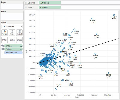
• Create a scatterplot of Profit vs. Sales per Product
• Add a Trend Line to the chart

Profit vs. Sales per Product

Step 2:

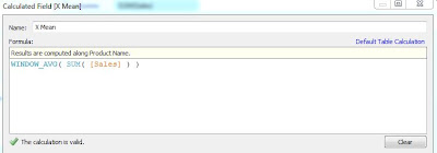
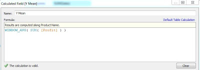
• Find the means for Sales and Profit
• Create the following calculated fields

X Mean (Sales)

Y Mean (Profit)

I labelled these X and Y instead of Sales and Profit because it makes it easier to remember where they go in the formulas.  You can name these anything you wish, as long as you know what they are.  Since this procedure is involved, it's always best to drag the values onto the Label Shelf to see if they are calculated properly.

Means (Test)

The means are the same for every point, and they seem to be reasonable values.  This is good enough for us.
Step 3:

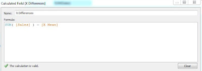
• Calculate the difference of each point from the mean for Sales and Profit, individually
• Create the following calculated fields

X Differences

Y Differences

Now, let's check our work.

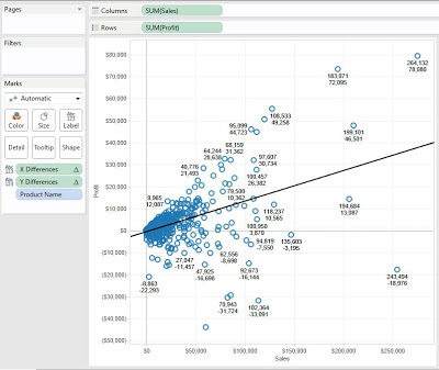
Differences (Test)

The values are different for each point, and get larger as they get further from the means.  Check #2 complete.

Step 4:

• Calculate the Sum of Squares for XX and XY
• Create the following calculated field

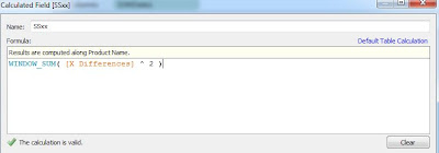
SSxx

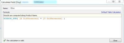
SSxy

We won't get into why these formulas are called Sum of Squares, or why they look the way they do.  Just know that these are the mathematically correct formulas.  Now, let's check our work.

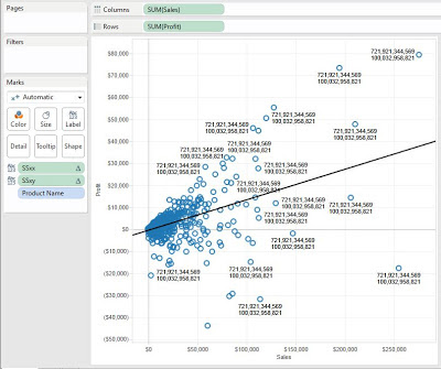
Sum of Squares (Test)

We can see that the values are the same for every point, and are really big (which is about all we can decipher from such a value).  Check #3 complete.

Step 5:

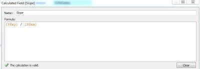
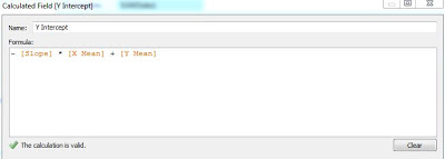
• Calculate the Slope and Y Intercept
• Create the following calculated fields

Slope

Y Intercept

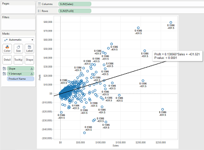
Finally, let's check to see if these values are the same as what Tableau calculates.

Slope and Intercept (Test)

Drawing back on high school, you might remember that Slope-Intercept form is y = mx + b.  We can see that our values match the values for the trend line.  Now, we can use these values for any other calculations.  Thanks for reading.  We hope you found this informative.

P.S.

For those of you that remember the Z-Test package we published to the Tableau forums a while ago, it has been updated to include this procedure as well.  We have also created another document describing this technique at http://community.tableausoftware.com/docs/DOC-1479.

Brad Llewellyn

Associate Consultant

Mariner, LLC

llewellyn.wb@gmail.com
https://www.linkedin.com/in/bradllewellyn