Azure Machine Learning Workbench: Utilizing Different Environments

Today, we're going to continue looking at the Azure Machine Learning (AML) Workbench.  In the previous post, we created a new Classifying_Iris project and walked through the basic layout of the Workbench.  In this post, we'll be walking through the rest of the code in the Quick CLI Reference section of the Dashboard.  This will focus on running our code utilizing different environments.

One of the biggest advantages of the cloud for modern data science is the ability to endlessly scale your resources in order to solve the problem at hand.  In some cases, like small-scale development, it's acceptable to run a process on our local machine.  However, as we need more processing power, we need to be able to run our code in more powerful environments, such as Azure Virtual Machines or HDInsight clusters.  Let's see how AML Workbench helps us accomplish this.

If you are new to the AML Workbench and haven't read the previous post, it is highly recommended that you do so.  The rest of this post will build on what we learned in the previous one.

Here's the first piece of code we will run.

az ml experiment submit -c local iris_sklearn.py

This code runs the "iris_sklearn.py" Python script using our local machine.  We'll cover exactly what this script does in a later post.  All we need to know for now is that it's running on our local machine using Python.  As we mentioned before, using the local machine is great if we're just trying to do something small without having to worry about connecting to remote resources.  Here's the output.

OUTPUT BEGIN

RunId: Classifying_Iris_1509458498714

Executing user inputs .....
===========================

Python version: 3.5.2 |Continuum Analytics, Inc.| (default, Jul  5 2016, 11:41:13) [MSC v.1900 64 bit (AMD64)]

Iris dataset shape: (150, 5)
Regularization rate is 0.01
LogisticRegression(C=100.0, class_weight=None, dual=False, fit_intercept=True,
          intercept_scaling=1, max_iter=100, multi_class='ovr', n_jobs=1,
          penalty='l2', random_state=None, solver='liblinear', tol=0.0001,
          verbose=0, warm_start=False)
Accuracy is 0.6792452830188679

==========================================
Serialize and deserialize using the outputs folder.

Export the model to model.pkl
Import the model from model.pkl
New sample: [[3.0, 3.6, 1.3, 0.25]]
Predicted class is ['Iris-setosa']
Plotting confusion matrix...
Confusion matrix in text:
[[50  0  0]
 [ 1 37 12]
 [ 0  4 46]]
Confusion matrix plotted.
Plotting ROC curve....
ROC curve plotted.
Confusion matrix and ROC curve plotted. See them in Run History details page.

Execution Details
=================

RunId: Classifying_Iris_1509458498714

OUTPUT END

Here's the next piece of code.

az ml experiment submit -c docker-python iris_sklearn.py

This code runs the same "iris_sklearn.py" script as before.  However, this time it uses a Python-enabled Docker container.  Docker is a technology that allows us package an entire environment into a single object.  This is extremely useful when we are trying to deploy code across distributed systems.  For instance, some organizations will wrap their applications in Docker containers, then deploy the Docker containers.  This allows them to manage the applications much easier because they can update the master Docker container, and that update can be automatically deployed to all of the existing Docker containers.  You can read more about Docker and containers here, here and here. Unfortunately, we're unable to install Docker on our machine.  So, we'll have to skip this one.  Let's take a look at the next piece of code.

az ml experiment submit -c docker-spark iris_pyspark.py

This code runs a new script called "iris_pyspark.py".  We'll save the in-depth analysis of the code for a later post.  To heavily summarize, PySpark is a way to harness the power of Spark's big data analytical functionality from within Python.  This can be extremely useful when we want to analyze or model big data problems without using a remote Spark cluster.  Let's take a look at the next piece of code.

az ml computetarget attach --name myvm --address <ip address or FQDN> --username <username> --password <pwd> --type remotedocker

az ml experiment prepare -c myvm

az ml experiment submit -c myvm iris_pyspark.py

This is where things start to get interesting.  Previously, we were running everything on our local machine.  This is great when data is small.  However, it becomes unusable when we need to point to larger data sources.  Fortunately, the AML Workbench allows us to attach to a remote virtual machine in cases where we need additional resources.

Another important thing to notice is that we were able to seemlessly run the same code on our local machine as we are running on the virtual machine.  This means that we can develop on small samples on our local machine, then effortlessly run the same code on a larger virtual machine when we want to test against a larger dataset.  This is exactly why containers are becoming so popular.  They make it effortless to move code from a less powerful environment, like a local machine, up to a more powerful one, like a large virtual machine.

Another advantage of this ability is that we can now manage resource costs by limiting virtual machine usage.  The entire team can share the same virtual machine, using it only when they need the extra power.  We can even turn the vm off when we aren't using it, saving even more money.  You can read more about Azure Virtual Machines here.

Let's move to the final piece of code.

az ml computetarget attach --name myhdi --address <ip address or FQDN of the head node> --username <username> --password <pwd> --type cluster

az ml experiment prepare -c myhdi

az ml experiment submit -c myhdi iris_pyspark.py

This code is expands on the same concepts as the previous one.  In some cases, we have very large resource needs.  In those cases, even a powerful virtual machine may not have enough juice.  For those cases, we can use containers to deploy to an Azure HDInsight cluster.  This will allow us to take the same code we ran on our local machine and execute it full-scale using the power of Hadoop.  You can read more about HDInsight clusters here.

This post has opened our eyes to the power and flexibility that the AML Workbench can provide.  While it's more complicated than using its AML Studio counterpart, the power and flexibility it provides via containers can make all the difference for some organizations.  Stay tuned for the next post where we'll walk through the built-in data preparation capabilities of the Azure Machine Learning Workbench.  Thanks for reading.  We hope you found this informative.

Brad Llewellyn
Data Science Consultant
Valorem
@BreakingBI
www.linkedin.com/in/bradllewellyn
llewellyn.wb@gmail.com

Azure Machine Learning Webinars

As some of you may know, we've been giving Azure Machine Learning presentations for about a year now.  As promised, we wanted to include links to the videos, as well as any supplemental material for the presentations.

Azure Machine Learning Studio: Making Data Science Easy(er)

https://www.youtube.com/watch?v=QMj_dL64xCA

There are no supplemental materials for this presentation.

Azure Machine Learning Studio: Four Tips from the Pros

https://www.youtube.com/watch?v=d25wmQ_dSQg

https://drive.google.com/open?id=12xodphzcK1Oy7TBDDSzHPXe8GIiBIgbr

R Code for Creating Interaction Features

<R CODE START>

#####################

## Import Data

#####################

ignore <- c("income")

dat1 <- maml.mapInputPort(1)

dat.full <- dat1[,-which(names(dat1) %in% ignore)]

dat2 <- maml.mapInputPort(2)

vars.dummy <- names(dat.full)

vars.orig <- names(dat2[,-which(names(dat2) %in% ignore)])

temp <- dat.full[,1]

dat.int <- data.frame(temp)

################################################

## Loop through all possible combinations

################################################

for(i in 1:(length(vars.dummy) - 1)){

    for(j in 2:length(vars.dummy)){

        var1 <- vars.dummy[i]

        var2 <- vars.dummy[j]

        

        base1 <- substr(var1, 1, regexpr("-", var1) - 1)

        base2 <- substr(var2, 1, regexpr("-", var2) - 1)

        

        if( base1 != base2 ){

            val1 <- dat.full[,which(names(dat.full) %in% var1)]

            val2 <- dat.full[,which(names(dat.full) %in% var2)]

            dat.int[,length(dat.int) + 1] <- val1 * val2

            names(dat.int)[length(dat.int)] <- paste(var1, " * ", var2)

        }

    }

}

###################

## Output Data

###################

dat.out <- data.frame(dat1, dat.int[,-1])

maml.mapOutputPort("dat.out");

<R CODE END>

SQL Code for Combining Tune Model Hyperparameters Results

<SQL CODE 1 START>

SELECT
    'Two-Class Locally Deep Support Vector Machine - Binning' AS [Model Type]
,'LD-SVM Tree Depth' AS [Par 1 Name]
,[LD-SVM Tree Depth] AS [Par 1 Value]
,'Lambda W' AS [Par 2 Name]
,[Lambda W] AS [Par 2 Value]
,'Lambda Theta' AS [Par 3 Name]
,[Lambda Theta] AS [Par 3 Value]
,'Lambda Theta Prime' AS [Par 4 Name]
,[Lambda Theta Prime] AS [Par 4 Value]
,'Sigma' AS [Par 5 Name]
,[Sigma] AS [Par 5 Value]
,'Num Iterations' AS [Par 6 Name]
,[Num Iterations] AS [Par 6 Value]
    ,'None' AS [Par 7 Name]
    ,'' AS [Par 7 Value]
,[Accuracy]
,[Precision]
,[Recall]
,[F-Score]
,[AUC]
,[Average Log Loss]
,[Training Log Loss]
,[Precision] * [Recall] AS [Precision * Recall]
FROM t1
UNION ALL
SELECT
'Two-Class Neural Network - Binning' AS [Model Type]
,'Learning rate' AS [Par 1 Name]
,[Learning rate] AS [Par 1 Value]
    ,'None' AS [Par 2 Name]
    ,0 AS [Par 2 Value]
,'Number of iterations' AS [Par 3 Name]
,[Number of iterations] AS [Par 3 Value]
,'None' AS [Par 4 Name]
,0 AS [Par 4 Value]
,'None' AS [Par 5 Name]
,0 AS [Par 5 Value]
,'None' AS [Par 6 Name]
,0 AS [Par 6 Value]
,'LossFunction' AS [Par 7 Name]
,[LossFunction] AS [Par 7 Value]
,[Accuracy]
,[Precision]
,[Recall]
,[F-Score]
,[AUC]
,[Average Log Loss]
,[Training Log Loss]
,[Precision] * [Recall] AS [Precision * Recall]
FROM t2
UNION ALL
SELECT
'Two-Class Decision Jungle - Replicate' AS [Model Type]
,'Number of optimization steps per decision DAG layer' AS [Par 1 Name]
,[Number of optimization steps per decision DAG layer] AS [Par 1 Value]
,'Maximum width of the decision DAGs' AS [Par 2 Name]
,[Maximum width of the decision DAGs] AS [Par 2 Value]
,'Maximum depth of the decision DAGs' AS [Par 3 Name]
,[Maximum depth of the decision DAGs] AS [Par 3 Value]
,'Number of decision DAGs' AS [Par 4 Name]
,[Number of decision DAGs] AS [Par 4 Value]
,'None' AS [Par 5 Name]
,0 AS [Par 5 Value]
,'None' AS [Par 6 Name]
,0 AS [Par 6 Value]
    ,'None' AS [Par 7 Name]
    ,'' AS [Par 7 Value]
,[Accuracy]
,[Precision]
,[Recall]
,[F-Score]
,[AUC]
,[Average Log Loss]
,[Training Log Loss]
,[Precision] * [Recall] AS [Precision * Recall]

FROM t3

<SQL CODE 1 END>


<SQL CODE 2 START>

SELECT
'Two-Class Locally Deep Support Vector Machine - Gaussian' AS [Model Type]
,'LD-SVM Tree Depth' AS [Par 1 Name]
,[LD-SVM Tree Depth] AS [Par 1 Value]
,'Lambda W' AS [Par 2 Name]
,[Lambda W] AS [Par 2 Value]
,'Lambda Theta' AS [Par 3 Name]
,[Lambda Theta] AS [Par 3 Value]
,'Lambda Theta Prime' AS [Par 4 Name]
,[Lambda Theta Prime] AS [Par 4 Value]
,'Sigma' AS [Par 5 Name]
,[Sigma] AS [Par 5 Value]
,'Num Iterations' AS [Par 6 Name]
,[Num Iterations] AS [Par 6 Value]
    ,'None' AS [Par 7 Name]
    ,'' AS [Par 7 Value]
,[Accuracy]
,[Precision]
,[Recall]
,[F-Score]
,[AUC]
,[Average Log Loss]
,[Training Log Loss]
,[Precision] * [Recall] AS [Precision * Recall]
FROM t1
UNION ALL
SELECT
'Two-Class Neural Network - Gaussian' AS [Model Type]
,'Learning rate' AS [Par 1 Name]
,[Learning rate] AS [Par 1 Value]
    ,'None' AS [Par 2 Name]
    ,0 AS [Par 2 Value]
,'Number of iterations' AS [Par 3 Name]
,[Number of iterations] AS [Par 3 Value]
,'None' AS [Par 4 Name]
,0 AS [Par 4 Value]
,'None' AS [Par 5 Name]
,0 AS [Par 5 Value]
,'None' AS [Par 6 Name]
,0 AS [Par 6 Value]
,'LossFunction' AS [Par 7 Name]
,[LossFunction] AS [Par 7 Value]
,[Accuracy]
,[Precision]
,[Recall]
,[F-Score]
,[AUC]
,[Average Log Loss]
,[Training Log Loss]
,[Precision] * [Recall] AS [Precision * Recall]
FROM t2
UNION ALL
SELECT
'Two-Class Decision Jungle - Bagging' AS [Model Type]
,'Number of optimization steps per decision DAG layer' AS [Par 1 Name]
,[Number of optimization steps per decision DAG layer] AS [Par 1 Value]
,'Maximum width of the decision DAGs' AS [Par 2 Name]
,[Maximum width of the decision DAGs] AS [Par 2 Value]
,'Maximum depth of the decision DAGs' AS [Par 3 Name]
,[Maximum depth of the decision DAGs] AS [Par 3 Value]
,'Number of decision DAGs' AS [Par 4 Name]
,[Number of decision DAGs] AS [Par 4 Value]
,'None' AS [Par 5 Name]
,0 AS [Par 5 Value]
,'None' AS [Par 6 Name]
,0 AS [Par 6 Value]
    ,'None' AS [Par 7 Name]
    ,'' AS [Par 7 Value]
,[Accuracy]
,[Precision]
,[Recall]
,[F-Score]
,[AUC]
,[Average Log Loss]
,[Training Log Loss]
,[Precision] * [Recall] AS [Precision * Recall]

FROM t3

<SQL CODE 2 END>


<SQL CODE 3 START>

SELECT
'Two-Class Locally Deep Support Vector Machine - Min-Max' AS [Model Type]
,'LD-SVM Tree Depth' AS [Par 1 Name]
,[LD-SVM Tree Depth] AS [Par 1 Value]
,'Lambda W' AS [Par 2 Name]
,[Lambda W] AS [Par 2 Value]
,'Lambda Theta' AS [Par 3 Name]
,[Lambda Theta] AS [Par 3 Value]
,'Lambda Theta Prime' AS [Par 4 Name]
,[Lambda Theta Prime] AS [Par 4 Value]
,'Sigma' AS [Par 5 Name]
,[Sigma] AS [Par 5 Value]
,'Num Iterations' AS [Par 6 Name]
,[Num Iterations] AS [Par 6 Value]
    ,'None' AS [Par 7 Name]
    ,'' AS [Par 7 Value]
,[Accuracy]
,[Precision]
,[Recall]
,[F-Score]
,[AUC]
,[Average Log Loss]
,[Training Log Loss]
,[Precision] * [Recall] AS [Precision * Recall]
FROM t1
UNION ALL
SELECT
'Two-Class Neural Network - Min-Max' AS [Model Type]
,'Learning rate' AS [Par 1 Name]
,[Learning rate] AS [Par 1 Value]
,'None' AS [Par 2 Name]
,0 AS [Par 2 Value]
,'Number of iterations' AS [Par 3 Name]
,[Number of iterations] AS [Par 3 Value]
,'None' AS [Par 4 Name]
,0 AS [Par 4 Value]
,'None' AS [Par 5 Name]
,0 AS [Par 5 Value]
,'None' AS [Par 6 Name]
,0 AS [Par 6 Value]
,'LossFunction' AS [Par 7 Name]
,[LossFunction] AS [Par 7 Value]
,[Accuracy]
,[Precision]
,[Recall]
,[F-Score]
,[AUC]
,[Average Log Loss]
,[Training Log Loss]
,[Precision] * [Recall] AS [Precision * Recall]
FROM t2
UNION ALL
SELECT
'Two-Class Boosted Decision Tree' AS [Model Type]
,'Number of leaves' AS [Par 1 Name]
,[Number of leaves] AS [Par 1 Value]
,'Minimum leaf instances' AS [Par 2 Name]
,[Minimum leaf instances] AS [Par 2 Value]
,'Learning rate' AS [Par 3 Name]
,[Learning rate] AS [Par 3 Value]
,'Number of trees' AS [Par 4 Name]
,[Number of trees] AS [Par 4 Value]
,'None' AS [Par 5 Name]
,0 AS [Par 5 Value]
,'None' AS [Par 6 Name]
,0 AS [Par 6 Value]
    ,'None' AS [Par 7 Name]
    ,'' AS [Par 7 Value]
,[Accuracy]
,[Precision]
,[Recall]
,[F-Score]
,[AUC]
,[Average Log Loss]
,[Training Log Loss]
,[Precision] * [Recall] AS [Precision * Recall]

FROM t3

<SQL CODE 3 END>


<SQL CODE 4 START>

SELECT
'Two-Class Decision Forest - Replicate' AS [Model Type]
,'Minimum number of samples per leaf node' AS [Par 1 Name]
,[Minimum number of samples per leaf node] AS [Par 1 Value]
,'Number of random splits per node' AS [Par 2 Name]
,[Number of random splits per node] AS [Par 2 Value]
,'Maximum depth of the decision trees' AS [Par 3 Name]
,[Maximum depth of the decision trees] AS [Par 3 Value]
,'Number of decision trees' AS [Par 4 Name]
,[Number of decision trees] AS [Par 4 Value]
,'None' AS [Par 5 Name]
,0 AS [Par 5 Value]
,'None' AS [Par 6 Name]
,0 AS [Par 6 Value]
    ,'None' AS [Par 7 Name]
    ,'' AS [Par 7 Value]
,[Accuracy]
,[Precision]
,[Recall]
,[F-Score]
,[AUC]
,[Average Log Loss]
,[Training Log Loss]
,[Precision] * [Recall] AS [Precision * Recall]
FROM t1
UNION ALL
SELECT
'Two-Class Averaged Perceptron' AS [Model Type]
,'Learning rate' AS [Par 1 Name]
,[Learning rate] AS [Par 1 Value]
,'Maximum number of iterations' AS [Par 2 Name]
,[Maximum number of iterations] AS [Par 2 Value]
,'None' AS [Par 3 Name]
,0 AS [Par 3 Value]
,'None' AS [Par 4 Name]
,0 AS [Par 4 Value]
,'None' AS [Par 5 Name]
,0 AS [Par 5 Value]
,'None' AS [Par 6 Name]
,0 AS [Par 6 Value]
    ,'None' AS [Par 7 Name]
    ,'' AS [Par 7 Value]
,[Accuracy]
,[Precision]
,[Recall]
,[F-Score]
,[AUC]
,[Average Log Loss]
,[Training Log Loss]
,[Precision] * [Recall] AS [Precision * Recall]
FROM t2
UNION ALL
SELECT
'Two-Class Support Vector Machine' AS [Model Type]
,'Number of iterations' AS [Par 1 Name]
,[Number of iterations] AS [Par 1 Value]
,'Lambda' AS [Par 2 Name]
,[Lambda] AS [Par 2 Value]
,'None' AS [Par 3 Name]
,0 AS [Par 3 Value]
,'None' AS [Par 4 Name]
,0 AS [Par 4 Value]
,'None' AS [Par 5 Name]
,0 AS [Par 5 Value]
,'None' AS [Par 6 Name]
,0 AS [Par 6 Value]
    ,'None' AS [Par 7 Name]
    ,'' AS [Par 7 Value]
,[Accuracy]
,[Precision]
,[Recall]
,[F-Score]
,[AUC]
,[Average Log Loss]
,[Training Log Loss]
,[Precision] * [Recall] AS [Precision * Recall]

FROM t3

<SQL CODE 4 END>


<SQL CODE 5 START>

SELECT
'Two-Class Decision Forest - Bagging' AS [Model Type]
,'Minimum number of samples per leaf node' AS [Par 1 Name]
,[Minimum number of samples per leaf node] AS [Par 1 Value]
,'Number of random splits per node' AS [Par 2 Name]
,[Number of random splits per node] AS [Par 2 Value]
,'Maximum depth of the decision trees' AS [Par 3 Name]
,[Maximum depth of the decision trees] AS [Par 3 Value]
,'Number of decision trees' AS [Par 4 Name]
,[Number of decision trees] AS [Par 4 Value]
,'None' AS [Par 5 Name]
,0 AS [Par 5 Value]
,'None' AS [Par 6 Name]
,0 AS [Par 6 Value]
    ,'None' AS [Par 7 Name]
    ,'' AS [Par 7 Value]
,[Accuracy]
,[Precision]
,[Recall]
,[F-Score]
,[AUC]
,[Average Log Loss]
,[Training Log Loss]
,[Precision] * [Recall] AS [Precision * Recall]
FROM t1
UNION ALL
SELECT
'Two-Class Logistic Regression' AS [Model Type]
,'OptimizationTolerance' AS [Par 1 Name]
,[OptimizationTolerance] AS [Par 1 Value]
,'L1Weight' AS [Par 2 Name]
,[L1Weight] AS [Par 2 Value]
,'L2Weight' AS [Par 3 Name]
,[L2Weight] AS [Par 3 Value]
,'MemorySize' AS [Par 4 Name]
,[MemorySize] AS [Par 4 Value]
,'None' AS [Par 5 Name]
,0 AS [Par 5 Value]
,'None' AS [Par 6 Name]
,0 AS [Par 6 Value]
    ,'None' AS [Par 7 Name]
    ,'' AS [Par 7 Value]
,[Accuracy]
,[Precision]
,[Recall]
,[F-Score]
,[AUC]
,[Average Log Loss]
,[Training Log Loss]
,[Precision] * [Recall] AS [Precision * Recall]

FROM t2

<SQL CODE 5 END>


<SQL CODE 6 START>

SELECT * FROM t1
UNION ALL
SELECT * FROM t2
UNION ALL

SELECT * FROM t3

<SQL CODE 6 END>


<SQL CODE 7 START>

SELECT * FROM t1
UNION ALL

SELECT * FROM t2

<SQL CODE 7 END>


<SQL CODE 8 START>

SELECT * FROM t1
UNION ALL

SELECT * FROM t2

<SQL CODE 8 END>

<SQL CODE 9 START>

SELECT * FROM t1
ORDER BY [AUC] DESC

<SQL CODE 9 END>

Brad Llewellyn
Data Science Consultant
Valorem
@BreakingBI
www.linkedin.com/in/bradllewellyn
llewellyn.wb@gmail.com

Azure Machine Learning Workbench: Getting Started

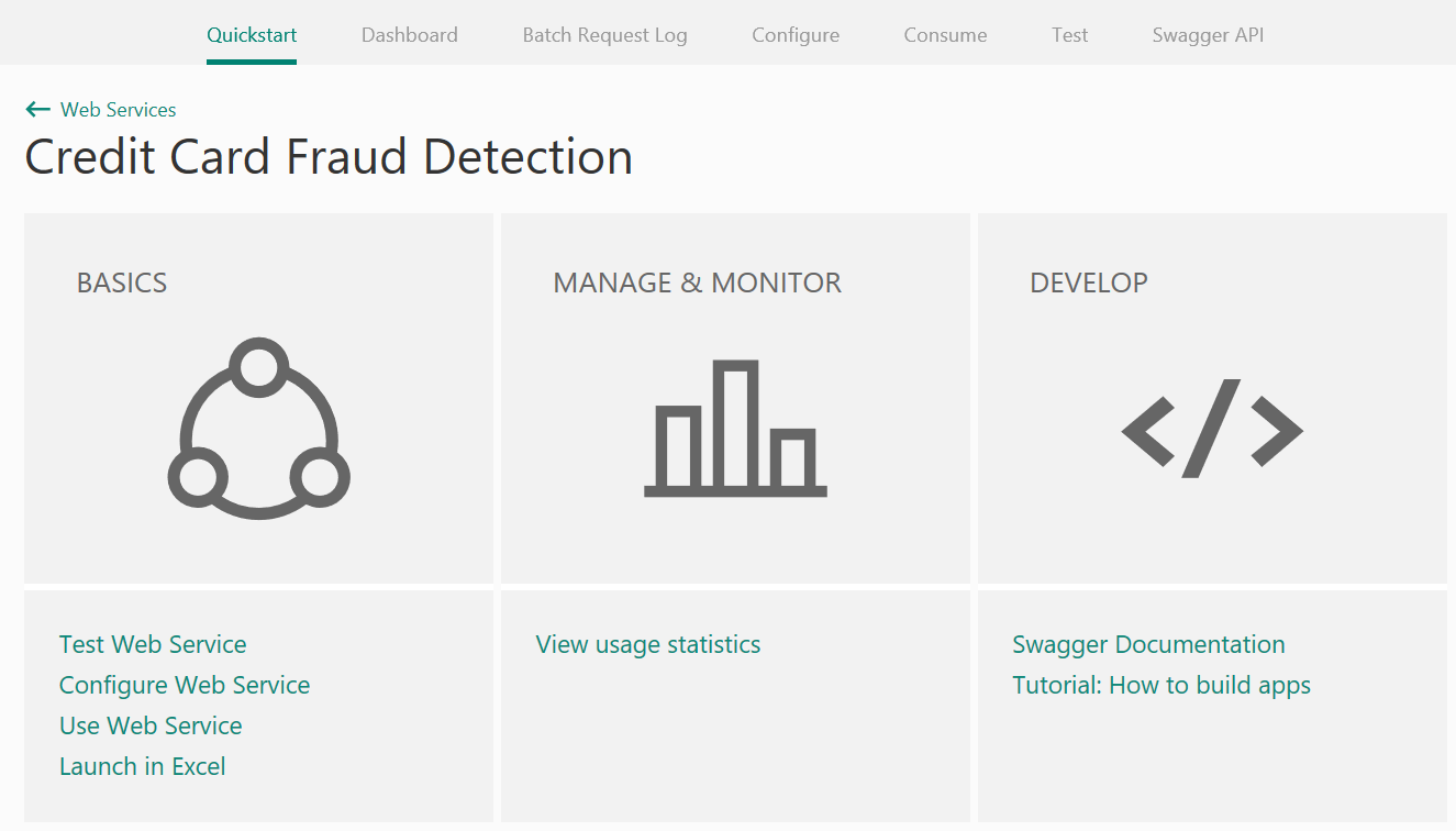
Today, we're going to take a look at one of the newest Data Science offerings from Microsoft.  Of course, we're talking about the Azure Machine Learning (AML) Workbench!  Join us as we dive in and see what this new tool is all about.

Before we install the AML Workbench, let's talk about what it is.  The AML Workbench is a local environment for developing data science solutions that can be easily deployed and managed using Microsoft Azure.  It doesn't appear to be related to AML Studio in any way.  Throughout this series, we'll walk through all of the different things we can do with the AML Workbench.  For today, we're just going to get our feet wet.

Now, we need to create an Azure Machine Learning Experimentation resource in the Azure portal.  You can find complete instructions here.  We will also include a Workspace and a Model Management Account.  This appears to be free for the first two users.  However, we're not sure whether they charge separately for the storage account.  Maybe someone can let us know in the comments.  Now, let's boot this baby up!

Azure Machine Learning Workbench

New Project

In the top-left corner, we can see the Workspace we created in the Azure portal.  Let's add a new Project to this.

Create New Project

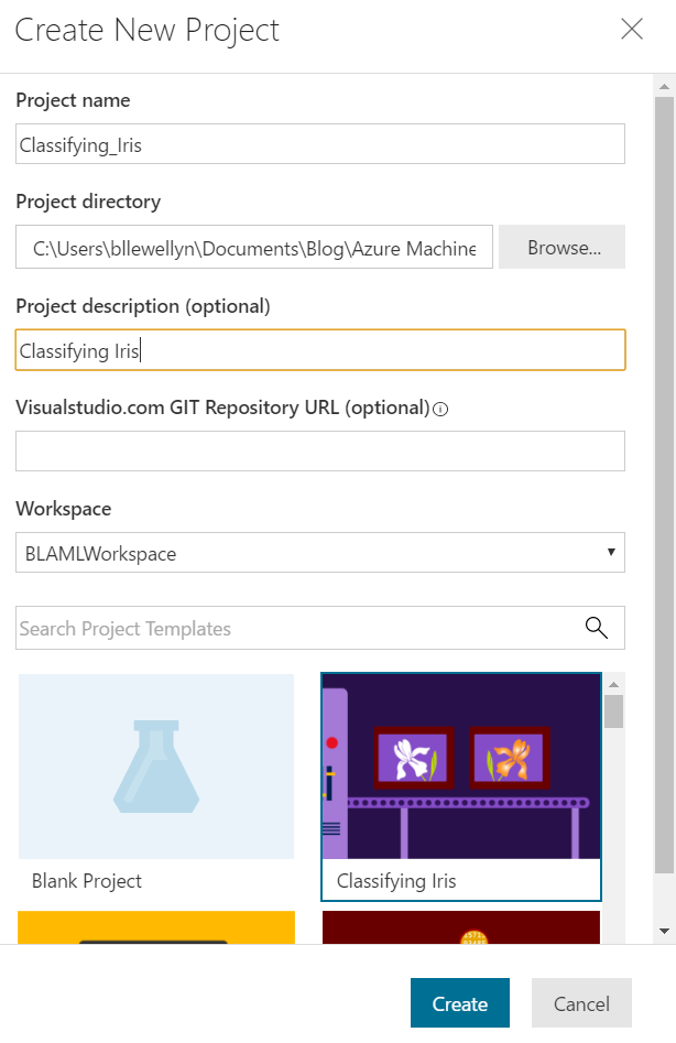
Now, we have to add the details for our new project.  Strangely, the project name can't include spaces.  We felt like we were past the point where names had to be simple, but maybe it's a Git thing.  Either way, we'll call our new project "Classifying_Iris" and use the "Classifying Iris" template at the bottom of the screen.  Let's see what's inside this project.

Project Dashboard

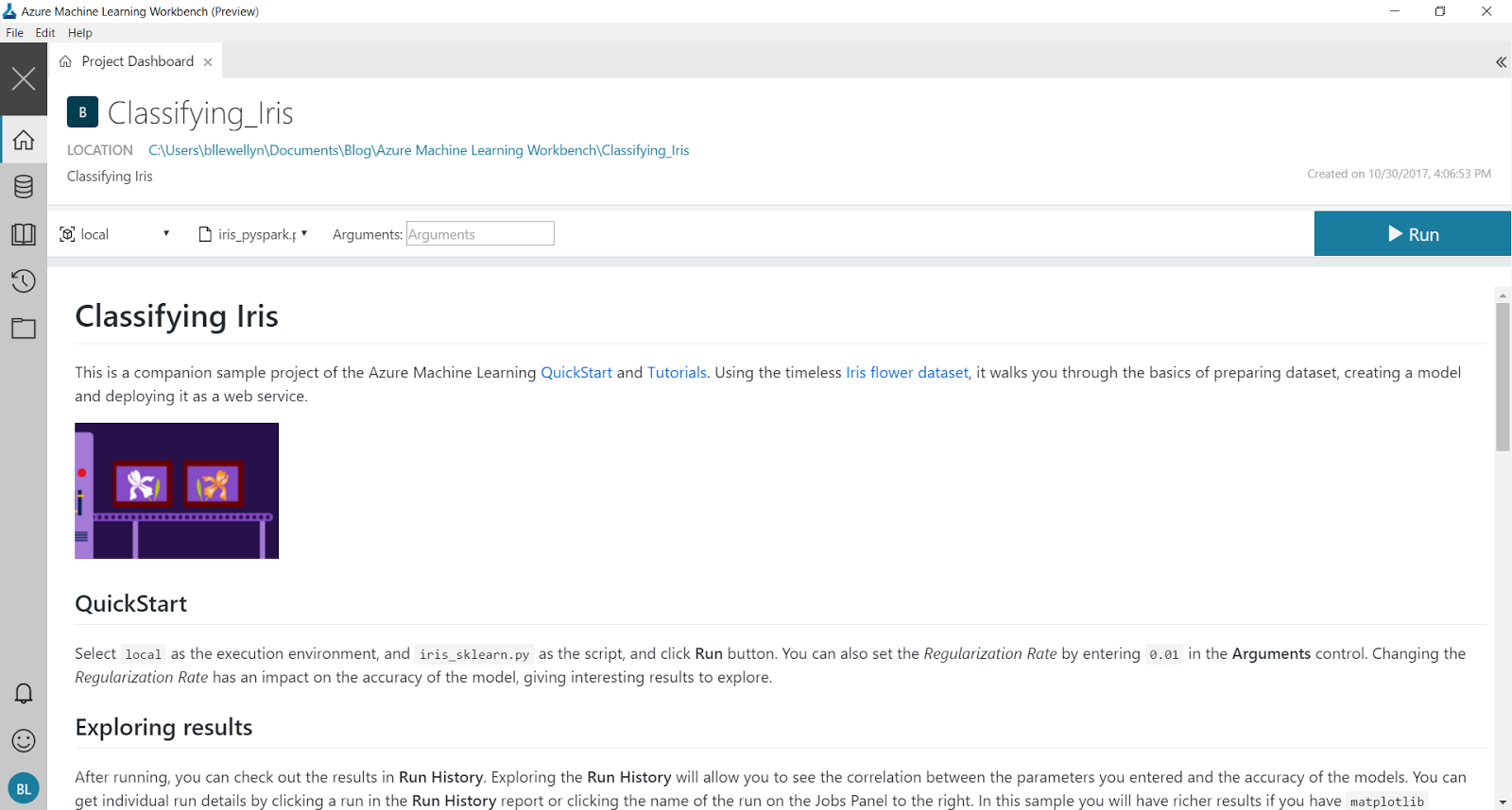
The first thing we see is the Project Dashboard.  This is a great place to create (or read) quality documentation on exactly what the project does, links to external resources, etc.

iris_sklearn

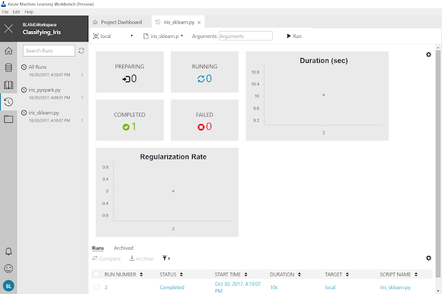
Following the QuickStart instructions, we were able to run the "iris_sklearn.py" code.  Unfortunately, it's not immediately obvious what this does.  Fortunately, the Exploring Results section tells us to check the Run History.  We can find this icon on the left side of the screen.

Run History

iris_sklearn Run History

This is pretty cool stuff actually.  This view would let us know how long our code is taking to run, as well as what parameters are being input.  This would be extremely helpful if we were running repeated experiments.  In our case, it doesn't show much though.

Job History

If we click on the Job Name in the Jobs section on the right side of the screen, we can see a more detailed result set.

Run Properties

This is what we were looking for!  This gives us all kinds of information about the run.  This could be extremely useful for showing the results of an experiment to bosses or colleagues.

Logs

Further down the page, we see the Logs section.  This is where we can access all the granular information we would need if we needed to debug a particular issue.

The next section of the instructions is the Quick CLI Reference.  This gives us a bunch of code we can use to run these scripts from the Command Line (or Powershell).  Let's open a new command line window.

Open Command Prompt

In the top-left corner of the window, we can select "Open Command Prompt" from the "File" menu.

Command Prompt

In the command prompt, we can copy the first line of code from the instructions.

pip install matplotlib

This code will install the Python library "matplotlib".  This library contains quite a few functions for creating graphs in Python.  You can read more about it here.  Now that we have the library installed, let's copy the next line of code.

az login

This code will help us log the Command Line Interface into Azure.  When we run this command, we get the following response.

To sign in, use a web browser to open the page https://aka.ms/devicelogin and enter the code ######### to authenticate.

When we follow the instructions, we can log into our Azure subscription.

Azure Login

The next piece of code we need to run is as follows.

python run.py

This piece of code will run the "run.py" script from our project.  We'll look at this script in a later post.  For now, let's see the output from this script.  Please note that the "run.py" script is iterative and creates a large amount of output.  You can skip to the OUTPUT END header if you don't want to see the output.

OUTPUT BEGIN

RunId: Classifying_Iris_1509457170414

Executing user inputs .....
===========================

Python version: 3.5.2 |Continuum Analytics, Inc.| (default, Jul  5 2016, 11:41:13) [MSC v.1900 64 bit (AMD64)]

Iris dataset shape: (150, 5)
Regularization rate is 10.0
LogisticRegression(C=0.1, class_weight=None, dual=False, fit_intercept=True,
          intercept_scaling=1, max_iter=100, multi_class='ovr', n_jobs=1,
          penalty='l2', random_state=None, solver='liblinear', tol=0.0001,
          verbose=0, warm_start=False)
Accuracy is 0.6415094339622641

==========================================
Serialize and deserialize using the outputs folder.

Export the model to model.pkl
Import the model from model.pkl
New sample: [[3.0, 3.6, 1.3, 0.25]]
Predicted class is ['Iris-setosa']
Plotting confusion matrix...
Confusion matrix in text:
[[50  0  0]
 [ 0 31 19]
 [ 0  4 46]]
Confusion matrix plotted.
Plotting ROC curve....
ROC curve plotted.
Confusion matrix and ROC curve plotted. See them in Run History details page.

Execution Details
=================
RunId: Classifying_Iris_1509457170414

RunId: Classifying_Iris_1509457188739

Executing user inputs .....
===========================

Python version: 3.5.2 |Continuum Analytics, Inc.| (default, Jul  5 2016, 11:41:13) [MSC v.1900 64 bit (AMD64)]

Iris dataset shape: (150, 5)
Regularization rate is 5.0
LogisticRegression(C=0.2, class_weight=None, dual=False, fit_intercept=True,
          intercept_scaling=1, max_iter=100, multi_class='ovr', n_jobs=1,
          penalty='l2', random_state=None, solver='liblinear', tol=0.0001,
          verbose=0, warm_start=False)
Accuracy is 0.6415094339622641

==========================================
Serialize and deserialize using the outputs folder.

Export the model to model.pkl
Import the model from model.pkl
New sample: [[3.0, 3.6, 1.3, 0.25]]
Predicted class is ['Iris-setosa']
Plotting confusion matrix...
Confusion matrix in text:
[[50  0  0]
 [ 0 32 18]
 [ 0  4 46]]
Confusion matrix plotted.
Plotting ROC curve....
ROC curve plotted.
Confusion matrix and ROC curve plotted. See them in Run History details page.

Execution Details
=================
RunId: Classifying_Iris_1509457188739

RunId: Classifying_Iris_1509457195895

Executing user inputs .....
===========================

Python version: 3.5.2 |Continuum Analytics, Inc.| (default, Jul  5 2016, 11:41:13) [MSC v.1900 64 bit (AMD64)]

Iris dataset shape: (150, 5)
Regularization rate is 2.5
LogisticRegression(C=0.4, class_weight=None, dual=False, fit_intercept=True,
          intercept_scaling=1, max_iter=100, multi_class='ovr', n_jobs=1,
          penalty='l2', random_state=None, solver='liblinear', tol=0.0001,
          verbose=0, warm_start=False)
Accuracy is 0.660377358490566

==========================================
Serialize and deserialize using the outputs folder.

Export the model to model.pkl
Import the model from model.pkl
New sample: [[3.0, 3.6, 1.3, 0.25]]
Predicted class is ['Iris-setosa']
Plotting confusion matrix...
Confusion matrix in text:
[[50  0  0]
 [ 0 33 17]
 [ 0  4 46]]
Confusion matrix plotted.
Plotting ROC curve....
ROC curve plotted.
Confusion matrix and ROC curve plotted. See them in Run History details page.

Execution Details
=================
RunId: Classifying_Iris_1509457195895

RunId: Classifying_Iris_1509457203051

Executing user inputs .....
===========================

Python version: 3.5.2 |Continuum Analytics, Inc.| (default, Jul  5 2016, 11:41:13) [MSC v.1900 64 bit (AMD64)]

Iris dataset shape: (150, 5)
Regularization rate is 1.25
LogisticRegression(C=0.8, class_weight=None, dual=False, fit_intercept=True,
          intercept_scaling=1, max_iter=100, multi_class='ovr', n_jobs=1,
          penalty='l2', random_state=None, solver='liblinear', tol=0.0001,
          verbose=0, warm_start=False)
Accuracy is 0.6415094339622641

==========================================
Serialize and deserialize using the outputs folder.

Export the model to model.pkl
Import the model from model.pkl
New sample: [[3.0, 3.6, 1.3, 0.25]]
Predicted class is ['Iris-setosa']
Plotting confusion matrix...
Confusion matrix in text:
[[50  0  0]
 [ 1 33 16]
 [ 0  5 45]]
Confusion matrix plotted.
Plotting ROC curve....
ROC curve plotted.
Confusion matrix and ROC curve plotted. See them in Run History details page.

Execution Details
=================
RunId: Classifying_Iris_1509457203051

RunId: Classifying_Iris_1509457210237

Executing user inputs .....
===========================

Python version: 3.5.2 |Continuum Analytics, Inc.| (default, Jul  5 2016, 11:41:13) [MSC v.1900 64 bit (AMD64)]

Iris dataset shape: (150, 5)
Regularization rate is 0.625
LogisticRegression(C=1.6, class_weight=None, dual=False, fit_intercept=True,
          intercept_scaling=1, max_iter=100, multi_class='ovr', n_jobs=1,
          penalty='l2', random_state=None, solver='liblinear', tol=0.0001,
          verbose=0, warm_start=False)
Accuracy is 0.660377358490566

==========================================
Serialize and deserialize using the outputs folder.

Export the model to model.pkl
Import the model from model.pkl
New sample: [[3.0, 3.6, 1.3, 0.25]]
Predicted class is ['Iris-setosa']
Plotting confusion matrix...
Confusion matrix in text:
[[50  0  0]
 [ 1 36 13]
 [ 0  5 45]]
Confusion matrix plotted.
Plotting ROC curve....
ROC curve plotted.
Confusion matrix and ROC curve plotted. See them in Run History details page.

Execution Details
=================
RunId: Classifying_Iris_1509457210237

RunId: Classifying_Iris_1509457217482

Executing user inputs .....
===========================

Python version: 3.5.2 |Continuum Analytics, Inc.| (default, Jul  5 2016, 11:41:13) [MSC v.1900 64 bit (AMD64)]

Iris dataset shape: (150, 5)
Regularization rate is 0.3125
LogisticRegression(C=3.2, class_weight=None, dual=False, fit_intercept=True,
          intercept_scaling=1, max_iter=100, multi_class='ovr', n_jobs=1,
          penalty='l2', random_state=None, solver='liblinear', tol=0.0001,
          verbose=0, warm_start=False)
Accuracy is 0.660377358490566

==========================================
Serialize and deserialize using the outputs folder.

Export the model to model.pkl
Import the model from model.pkl
New sample: [[3.0, 3.6, 1.3, 0.25]]
Predicted class is ['Iris-setosa']
Plotting confusion matrix...
Confusion matrix in text:
[[50  0  0]
 [ 1 36 13]
 [ 0  4 46]]
Confusion matrix plotted.
Plotting ROC curve....
ROC curve plotted.
Confusion matrix and ROC curve plotted. See them in Run History details page.

Execution Details
=================
RunId: Classifying_Iris_1509457217482

RunId: Classifying_Iris_1509457225704

Executing user inputs .....
===========================

Python version: 3.5.2 |Continuum Analytics, Inc.| (default, Jul  5 2016, 11:41:13) [MSC v.1900 64 bit (AMD64)]

Iris dataset shape: (150, 5)
Regularization rate is 0.15625
LogisticRegression(C=6.4, class_weight=None, dual=False, fit_intercept=True,
          intercept_scaling=1, max_iter=100, multi_class='ovr', n_jobs=1,
          penalty='l2', random_state=None, solver='liblinear', tol=0.0001,
          verbose=0, warm_start=False)
Accuracy is 0.6792452830188679

==========================================
Serialize and deserialize using the outputs folder.

Export the model to model.pkl
Import the model from model.pkl
New sample: [[3.0, 3.6, 1.3, 0.25]]
Predicted class is ['Iris-setosa']
Plotting confusion matrix...
Confusion matrix in text:
[[50  0  0]
 [ 1 36 13]
 [ 0  3 47]]
Confusion matrix plotted.
Plotting ROC curve....
ROC curve plotted.
Confusion matrix and ROC curve plotted. See them in Run History details page.

Execution Details
=================
RunId: Classifying_Iris_1509457225704

RunId: Classifying_Iris_1509457234132

Executing user inputs .....
===========================

Python version: 3.5.2 |Continuum Analytics, Inc.| (default, Jul  5 2016, 11:41:13) [MSC v.1900 64 bit (AMD64)]

Iris dataset shape: (150, 5)
Regularization rate is 0.078125
LogisticRegression(C=12.8, class_weight=None, dual=False, fit_intercept=True,
          intercept_scaling=1, max_iter=100, multi_class='ovr', n_jobs=1,
          penalty='l2', random_state=None, solver='liblinear', tol=0.0001,
          verbose=0, warm_start=False)
Accuracy is 0.6792452830188679

==========================================
Serialize and deserialize using the outputs folder.

Export the model to model.pkl
Import the model from model.pkl
New sample: [[3.0, 3.6, 1.3, 0.25]]
Predicted class is ['Iris-setosa']
Plotting confusion matrix...
Confusion matrix in text:
[[50  0  0]
 [ 1 36 13]
 [ 0  3 47]]
Confusion matrix plotted.
Plotting ROC curve....
ROC curve plotted.
Confusion matrix and ROC curve plotted. See them in Run History details page.

Execution Details
=================
RunId: Classifying_Iris_1509457234132

RunId: Classifying_Iris_1509457242301

Executing user inputs .....
===========================

Python version: 3.5.2 |Continuum Analytics, Inc.| (default, Jul  5 2016, 11:41:13) [MSC v.1900 64 bit (AMD64)]

Iris dataset shape: (150, 5)
Regularization rate is 0.0390625
LogisticRegression(C=25.6, class_weight=None, dual=False, fit_intercept=True,
          intercept_scaling=1, max_iter=100, multi_class='ovr', n_jobs=1,
          penalty='l2', random_state=None, solver='liblinear', tol=0.0001,
          verbose=0, warm_start=False)
Accuracy is 0.6981132075471698

==========================================
Serialize and deserialize using the outputs folder.

Export the model to model.pkl
Import the model from model.pkl
New sample: [[3.0, 3.6, 1.3, 0.25]]
Predicted class is ['Iris-setosa']
Plotting confusion matrix...
Confusion matrix in text:
[[50  0  0]
 [ 1 37 12]
 [ 0  3 47]]
Confusion matrix plotted.
Plotting ROC curve....
ROC curve plotted.
Confusion matrix and ROC curve plotted. See them in Run History details page.

Execution Details
=================
RunId: Classifying_Iris_1509457242301

RunId: Classifying_Iris_1509457249742

Executing user inputs .....
===========================

Python version: 3.5.2 |Continuum Analytics, Inc.| (default, Jul  5 2016, 11:41:13) [MSC v.1900 64 bit (AMD64)]

Iris dataset shape: (150, 5)
Regularization rate is 0.01953125
LogisticRegression(C=51.2, class_weight=None, dual=False, fit_intercept=True,
          intercept_scaling=1, max_iter=100, multi_class='ovr', n_jobs=1,
          penalty='l2', random_state=None, solver='liblinear', tol=0.0001,
          verbose=0, warm_start=False)
Accuracy is 0.6981132075471698

==========================================
Serialize and deserialize using the outputs folder.

Export the model to model.pkl
Import the model from model.pkl
New sample: [[3.0, 3.6, 1.3, 0.25]]
Predicted class is ['Iris-setosa']
Plotting confusion matrix...
Confusion matrix in text:
[[50  0  0]
 [ 1 37 12]
 [ 0  3 47]]
Confusion matrix plotted.
Plotting ROC curve....
ROC curve plotted.
Confusion matrix and ROC curve plotted. See them in Run History details page.

Execution Details
=================
RunId: Classifying_Iris_1509457249742

RunId: Classifying_Iris_1509457257076

Executing user inputs .....
===========================

Python version: 3.5.2 |Continuum Analytics, Inc.| (default, Jul  5 2016, 11:41:13) [MSC v.1900 64 bit (AMD64)]

Iris dataset shape: (150, 5)
Regularization rate is 0.009765625
LogisticRegression(C=102.4, class_weight=None, dual=False, fit_intercept=True,
          intercept_scaling=1, max_iter=100, multi_class='ovr', n_jobs=1,
          penalty='l2', random_state=None, solver='liblinear', tol=0.0001,
          verbose=0, warm_start=False)
Accuracy is 0.6792452830188679

==========================================
Serialize and deserialize using the outputs folder.

Export the model to model.pkl
Import the model from model.pkl
New sample: [[3.0, 3.6, 1.3, 0.25]]
Predicted class is ['Iris-setosa']
Plotting confusion matrix...
Confusion matrix in text:
[[50  0  0]
 [ 1 37 12]
 [ 0  4 46]]
Confusion matrix plotted.
Plotting ROC curve....
ROC curve plotted.
Confusion matrix and ROC curve plotted. See them in Run History details page.

Execution Details
=================

RunId: Classifying_Iris_1509457257076

OUTPUT END

Like we said before, we'll dig more into this code in a later post.  For now, let's take a look at the run history again.

Run History 2

Now, we can see all of the runs that just took place.  This is a really easy way to get a visual of what our code was accomplishing.

This seems like a good place to stop for today.  At first glance, the AML Workbench is much more developer-oriented than its Studio counterpart.  There's a ton of information here, but it's going to take some more time for us to get comfortable here.  Stay tuned for the next post where we'll dig into the rest of the pre-built code focusing on executing our code in different environments.  Thanks for reading.  We hope you found this informative.

Brad Llewellyn
Data Science Consultant
Valorem
@BreakingBI
www.linkedin.com/in/bradllewellyn
llewellyn.wb@gmail.com

Azure Machine Learning in Practice: Productionalization

Today, we're going to finish up our Fraud Detection experiment.  If you haven't read our previous posts in this series, it's recommended that you do so.  They cover the Preparation, Data Cleansing, Model Selection, Model Evaluation, Threshold Selection, Feature Selection and Feature Engineering phases of the experiment.  In this post, we're going to walk through the Productionalization process.

Productionalization is the process of taking the work we've done so far and making it accessible to the end user.  This is by far the most important process.  If we are unable to connect the end user to the model, then everything up until now was for nothing.  Fortunately, this is where Azure Machine Learning really differentiates itself from the rest of the data science tools on the market.  First, let's create a simple experiment that takes our testing data and scores that data using our trained model.  Remember that we investigated the use of some basic engineered features, but found that they didn't add value.

Productionalization

Now, let's take a minute to talk about web services.  A web service is a simple resource that sits on the Internet.  A user or application can send a set of data to this web service and receive a set of data in return, assuming they have the permissions to do so.  In our case, Azure Machine Learning makes it incredibly simple to create a deploy our experiement as an Azure Web Service.

Set Up Web Service

On the bar at the bottom of the Azure Machine Learning Studio, there's a button for "Set Up Web Service".  If we click it, we get a neat animation and a few changes to our experiment.

Predictive Experiment

We can see that we now have two new modules, "Web Service Input" and "Web Service Output".  When the user or application hits the web service, these are what they interact with.  The user or application passes a data set to the web service as a JSON payload.  Then, that payload flows into our Predictive Experiment and is scored using our model.  Finally, that scored data set is passed back to the user or application as a JSON payload.  The simplicity and flexibility of this type of model means that virtually any environment can easily integrate with Azure Machine Learning experiments.  However, we need to deploy it first.

Deploy Web Service

Just like with creating the web service, deployment is as easy as clicking a button on the bottom bar.  Unless you have a reason, it's good practice to deploy a new web service, as opposed to a classic one.

Web Service Deployment

Now, all we have to do is link it to a web service plan and we're off!  You can find out more about web service plans and their pricing here.  Basically, you can pay-as-you-go or you can buy a bundle at a discount and pay for any overges.  Now, let's take a look at a brand new portal, the Azure Machine Learning Web Services Portal.

Azure Machine Learning Web Services Portal

This is where we can manage and monitor all of of our Azure Machine Learning Web Services.  We'll gloss over this for now, as it's not the subject of this post.  However, we may venture back in a later post.  Let's move over to the "Consume" tab.

Azure Machine Learning Web Service Consumption Information

On this tab, we can find the keys and URIs for our new web services.  However, there's something far more powerful lurking further down on the page.

Sample Web Service Code

Azure Machine Learning provides sample code for calling the web service using four languages, C#, Python, Python 3+ and R.  This is amazing for us because we're not developers.  We couldn't code our way out of a box.  But, Azure Machine Learning makes it so easy that we don't have to.

Hopefully, this post sparked your imagination for all the ways that you could utilize Azure Machine Learning in your organization.  Azure Machine Learning is one of the best data science tools on the market because it drastically slashes the amount of time it takes to build, evaluate and productionalize your machine learning algorithms.  Thanks for reading.  We hope you found this informative.

Brad Llewellyn
Data Science Consultant
Valorem
@BreakingBI
www.linkedin.com/in/bradllewellyn
llewellyn.wb@gmail.com

Azure Machine Learning in Practice: Feature Selection

Today, we're going to continue with our Fraud Detection experiment.  If you haven't read our previous posts in this series, it's recommended that you do so.  They cover the Preparation, Data Cleansing, Model Selection, Model Evaluation and Threshold Selection phases of the experiment.  In this post, we're going to walk through the feature selection process.

In the traditional data science space, feature selection is generally one of the first phases of a modelling process.  A large reason for this is that, historically, building models using a hundred features would take a long time.  Also, an individual would have to sort through all of the features after modeling to determine what impact the features were having.  Sometimes, they would even find that some features would make the model less accurate by including them.  There's also the concept of parsimony to consider.  Basically, less variables was generally considered better.

However, technology and modelling techniques have come a long way over the last few decades.  We would be doing a great disservice to modern Machine Learning to say that it resembles traditional statistics in a major way.  Therefore, we try to approach feature selection from a more practical perspective.

First, we found that we were able to train over 1000 models in about an hour and a half.  Therefore, removing features for performance reasons is not necessary.  However, in other cases, it may be.  In those cases, paring down features initially could be beneficial.

Now, we need to determine which variables are having no (or even negative) impact on the resulting model.  If they aren't helping, then we should remove them.  To do this, we can use a technique known as Permutation Feature Importance.  Azure Machine Learning even has a built-in module for this.  Let's take a look.

Feature Selection Experiment

Permutation Feature Importance

This module requires us to input our trained model, as well as a testing dataset.  We also have to decide which metric we would like to use.  With that, it will output a dataset showing us the impact that each feature has on the model.

So, how does Permutation Feature Importance work?  Honestly, it's one of more clever algorithms we've come across.  The module chooses one feature at a time, randomly shuffles the values for that feature across the different rows, then retrains the model.  Then, it can evaluate the impact of that feature by seeing how much the trained model changed when the values were shuffled.  A very important feature would obviously cause large changes in the model if they were shuffled.  A less important feature would have less impact.  In our case, we want to measure impact by using Precision and Recall.  Unfortunately, the module only gives us the option to use one at a time.  Therefore, we'll have to be more creative.  Let's start by looking at the output of the Precision module.

Feature Importance (Precision) 1

Feature Importance (Precision) 2

We can see that there a few features that are important.  The rest of the features have no impact on the model.  Let's look at the output from the Recall module.

Feature Importance (Recall) 1

Feature Importance (Recall) 2

Now, let's compare the results of the two modules.

Feature Importance

We can see that the two modules have almost the same output, except for V4, which is only important for Precision.  This means that we should be able to remove all of the other features without affecting the model.  Let's try it and see what happens.

Feature Reduction Experiment

Tune Model Hyperparameters Results

R Script Results

We can see that removing those features from the model did reduce the Precision and Recall.  There was not a dramatic reduction in these values, but there was a reduction nonetheless.  This is likely caused by rounding error.  What was originally a very small decimal value assigned to the importance of each feature was rounded to 0, causing us to think that there was no importance.  Therefore, we are at a decision point.  Do we remove the features knowing that they slightly hurt the model?  Since we're having no performance issues and model understandability is not a factor, we would say no.  It's better to keep the original model than it is to make a slimmer version.

It is important to note that in practice, we've never seen the "Permutation Feature Importance" model throw out the majority of the features.  Usually, there are a few features that have a negative impact.  As we slowly remove them one at a time, we eventually find that most of the features have a positive impact on the model.  While we won't get into the math behind the scenes, we will say that we highly suspect this unusual case was caused by the fact that we are only given a subset of the Principal Components created using Principal Components Analysis.

Hopefully, this post enlightened you to some of the thought process behind Feature Selection in Azure Machine Learning.  Permutation Feature Importance is a fast, simple way to improve the accuracy and performance of your model.  Stay tuned for the next post where we'll be talking about Feature Engineering.  Thanks for reading.  We hope you found this informative.

Brad Llewellyn
Data Scientist
Valorem
@BreakingBI
www.linkedin.com/in/bradllewellyn
llewellyn.wb@gmail.com