Monday, September 30, 2013

Tableau vs. Power Pivot Part 3: Basic Data Modeling

Today, we will talk about how to handle data modeling in Power Pivot and Tableau.  In order to do this, we need to talk about the difference between "Joining" (Power Pivot) and "Blending" (Tableau).  A join is a static relationship that is reused over and over again for every calculation, with the exception of the ones you specifically code to reject that relationship.  Blending is a dynamic relationship that is used for one chart and one chart only.  Here's a simple example.

Imagine you have a fact table of sales per day with standard mm/dd/yyyy dates.  You also have a fully functional date dimension.  For those of you that don't know what a date dimension is,  it's a table where you can find all of the information about a date.  Some example information would be Month, Year, Weekday/Weekend, Fiscal Quarter, Holiday Status, etc.  Here's a simple example of a date dimension.
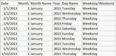
Date Dimension
Your goal is to report using the data from the main table, but the Month Name from the date table.  Now, if you wanted to "Join" these tables, you would want to join at the lowest possible level, i.e. the day.  This is so that you maintain as much information as possible in this STATIC relationship.  However, if you were to "Blend" these tables, you would only blend at the level you needed.  So, if you wanted to report on Sales per Month, you would still "Join" at the day level, but you would "Blend" at the Month level.  This is actually quite a neat feature.  If you wanted a report that shows the day level, the month level, and the year level (in different charts), you would have to "Join" at the day level, but you could "Blend" each chart at it's respective level.  I have created a picture to illustrate this point.
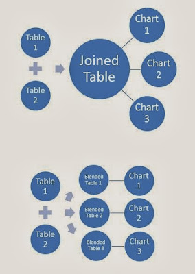
Joining vs. Blending

Now, let's get to the examination.

1 Fact and 1 Dimension

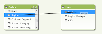
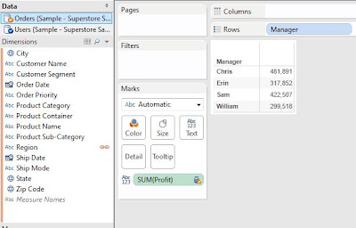
Here, we have a dimension that shows the managers for each Region and the CEO, who is over all Regions.  Let's see how easy it is to report on Profit by Region Manager.
Orders to Users on Region (Power Pivot)
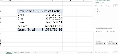
In order to define a relationship in Power Pivot, all you have to do is drag Region from Orders onto Region from Users.  Now, we can report on Sales by Region Manager.
Profit by Region Manager (Power Pivot)
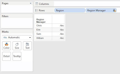
After creating the relationship, this was just as simple as if there were in the same table.  Now, let's see what Tableau thinks.
Profit by Region Manager (Tableau)
First, I had to drag Manager and Profit onto the chart.  However, since there's no Manager field in the Orders table, I had to click on the "Chain" beside Region to get it to blend on Region.  This would have been a much more complex task in Tableau 7.  However, Tableau 8 has had some serious changes to the way it blends.  In this case, both of the procedures were almost identical.

Winner: Tie

1 Fact and 3 Dimensions

Now, let's add a list of Returned orders as well as a Date dimension to the mix.  Let's see how well we can see how many orders were returned for each Region Manager in 2012.
Orders to Users, Returns, and Date (Power Pivot)
This design is what is typically called a Star Schema.  A star schema is widely considered, at least in my experience, to be the gold standard for analytical data modeling.  If you want to know more about Star Schema, check out the Wikipedia article, which pays homage to Ralph Kimball, the "father" of the Star Schema.

In Power Pivot, creating this was just a few drags.  However, before we can go to the pivot table, we have to create our measure.  In a Star Schema, the measures typically originate in the Fact table.  Therefore, we need to flag which orders were returned from inside the Fact Table.
Returned? (Power Pivot)
Now, we will need to find a way to count the number of distinct orders that had returns.  To do this, we can add another calculated column.
Returned Order ID (Power Pivot)
Now, we need to create a calculated field that performs a distinct count on this column and subtracts 1 to account for the zeros.
Distinct Count of Returned Orders (Power Pivot)
Finally, we can create our pivot table.
Number of Returned Orders by Region Manager in 2012 (Power Pivot)
This was a mess.  It required a decent knowledge of how Power Pivot worked.  The reason we had to distinct count was because the Orders table is at the Order Line level, and we wanted to know how many Orders were returned.  Let's see how Tableau handles this.  The first thing we need to realize is that we need to prep a chart BEFORE we start creating calculations.  This is the opposite of the way Power Pivot does things.  First, let's pull out our Region Managers.
Region Managers (Tableau)
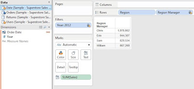
In order to keep the Orders table as the primary table, we had to put Region on the Chart, then hide it's header.  Then, we can put Region Manager on the chart.  Next, let's filter by Year.
Region Managers in 2012 (Tableau)
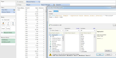
We have to drag Year onto the Filters Shelf and click the chain next to Order Date to ensure the connection.  We also have SUM( [Sales] ) on the chart so that we can be sure things are working the way we think they are.  Now, here's where Tableau differs from Power Pivot.  In order to properly calculate the returns, we must have Order ID on the chart.  We will just have to hide it later.  We can also create the same calculation we had in Power Pivot.
Returned? (Tableau)
Now, we need to hide the Order IDs and aggregate the chart up to the Region Manager level.  First, we need to calculate the total number of returned orders per Region Manager.
Sum of Returned (Tableau)
Sum of Returned Compute Using (Tableau)
Now, we have the number of returned orders per Region Manager.  The last thing we need to do is aggregate out the Order ID's.
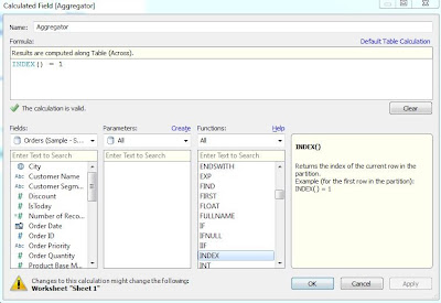
Aggregator (Tableau)
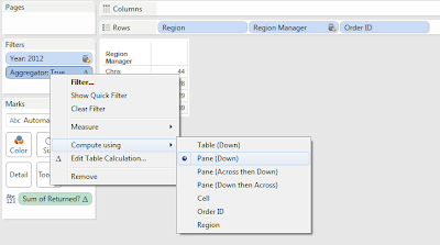
Aggregator (Compute Using)
Avid readers of this blog will recognize this technique.  However, it is not a beginner's technique.  Now, let's look at our final chart.
Number of Returned Orders by Region Manager in 2012 (Tableau)
These are the same numbers we saw in the Power Pivot table.  This leads us to believe that they are correct.  Looking back at this, the Power Pivot example required a beginner's knowledge of Power Pivot, while the Tableau example required an expert's knowledge of Tableau.  These examples took us about the same amount of time to do.  However, the beginner would likely struggle greatly with the Tableau version of this task.  Therefore, Power Pivot wins this section easily.

Winner: Power Pivot

Summary

This was a great exercise.  It showed that Tableau can handle basic data modeling.  However, as the models get more complex, Power Pivot begins to show its strengths.  We hope you found this informative.  Thanks for reading.

EDIT:  Zen Master Jonathan Drummey pointed out that we gave credit to Power Pivot's drag-and-drop joining feature, but did not do the same justice for Tableau.  Since Tableau's point-and-click joining mechanic is very powerful for Tableau, it should have been included in this post and we will utilize it in an upcoming post about advanced data modeling.  In fact, it would have made the solution a great deal simpler for the second section.

Brad Llewellyn
Associate Data Analytics Consultant
Mariner, LLC
brad.llewellyn@mariner-usa.com
http://www.linkedin.com/in/bradllewellyn
http://breaking-bi.blogspot.com

Monday, September 23, 2013

Tableau vs. Power Pivot Part 2: Basic Charting

Today, we will talk about creating basic charts in Tableau and Power Pivot.  To be specific, Power Pivot cannot create charts.  In order to create charts out of Power Pivot, you must either use Excel or Power View.  We will examine both of these as options.  As usual, we will use the Superstore Sales sample data set from Tableau.

Bar Graph (1 measure by 1 dimension)

The bar graph is most common of chart types and is useful for almost any type of analysis.  So, let's look at Profit by Region.
Profit by Region (Bar) (Excel)
This wasn't too hard in Excel.  However, it required us to first create the pivot table, then create the chart.  The labels and axes are also somewhat lacking.  More effort would have to be put into this to make it presentable.  Let's see how Power View fares.
Profit by Region (Bar) (Power View)
This was much easier than Excel.  The drag-and-drop interface makes everything much easier.  Also, the labels are very intuitive.  The graph is more aesthetically pleasing as well.  The only issue was that I had to resize the chart to see it all.  Finally, let's check out Tableau.
Profit by Region (Bar) (Tableau)
This was even easier than Power View.  I created this graph in two clicks, compared to four in Power View and much more in Excel.  I would say the aesthetics between Tableau and Power View are about equal.  This is the power behind these two tools after all.  It seems that Tableau has edged this one out ever so slightly.

Winner: Tableau

Bar Graph (1 measure by 2 dimensions)

Due to their interpretability, let's stay with bar graphs.  However, let's crank it up a notch and add a second dimension.  Let's see what Profit by Region and Category gives us.
Profit by Region and Category (Bar) (Excel)
Again, this wasn't too difficult.  Excel chose the roles intuitively, putting Region on the Rows and Category on the Colors.  This still required us to create the pivot table independent of the chart.  Also, we're still not impressed with the aesthetics or labels of the chart.  Finally, the label for the colors doesn't automatically appear, which could lead to confusion.  Let's see what Power View offers.
Profit by Region and Category (Bar) (Power View)
Just like last time, this was just a couple of clicks.  The labels and the aesthetics are acceptable.  My only concern about this chart is that the colors are a little too eye-catching for my taste.  A slightly softer palette would be nice in this case.  Now, on to Tableau.
Profit by Region and Category (Bar) (Tableau)
This was actually more complex than Power View.  In Power View, all I had to do was drag Category to the Legend Shelf.  In Tableau, I had to drag it to both the Rows Shelf and the Colors Shelf.  To our knowledge, Tableau is incapable of making clustered bar graphs.  This is probably our biggest frustration with Tableau.  How can a tool that is so good as visualizations lack such a simple feature?  Alas, we digress.  The point is this: not only was this chart more complex to make in Tableau than in Power View, it looks pretty unappealing.  As much as it pains me (a Tableau fanboy) to say it, Power View wins this one pretty convincingly.

Winner: Power View

Scatterplot (2 measures by 2 dimensions)

Now we're getting to the neat stuff.  How well can these tools handle dense graphs?  Let's try plotting Sales and Profit by Region and Customer (A hierarchical relationship!).
Sales and Profit by Region and Customer (Scatterplot) (Excel)
Turns out, Excel can't even do this (at least not simply).  This is all we needed to see.  Moving on to Power View.
Sales and Profit by Region and Customer (Scatterplot) (Power View)
This wasn't a very difficult task in Power View.  We also like the aesthetics of the graph.  All-in-all, this isn't a bad chart.  However, one of our biggest concerns with Power View is that it shows representative samples when the amount of points gets large.  This makes outlier detection nearly impossible.  If there is a way to turn this off, we haven't found it.  This being said, Power View doesn't seem to be a good tool for this type of chart.  Let's see what Tableau offers.
Sales and Profit by Region and Customer (Scatterplot) (Tableau)
This chart was no more difficult to make than the Power View chart.  However, it shows all the points.  Notice all of those outliers in the top-right of the chart?  We were missing most of those in the Power View chart.  Also, this graph just looks slightly cleaner to us.  Looking at this, it's easy to say that Tableau is the winner here.

Winner: Tableau

Mapping (1 measure by 1 geographic dimension)

Mapping is a newer type of technology that is becoming more mainstream.  Let's see how these tools handle it.  We'll try Profit by State.
Profit by State (Map) (Excel)
We couldn't even find a mapping feature in Excel.  If it's there, it's wasn't obvious to us.  Now, let's look at Power View.
Profit by State (Map) (Power View)
This wasn't a complex task in Power View.  However, the points can only be displayed as pie charts, or circles in this case.  Also, the points can only be colored by a dimension, not an automatically discretized measure.  This chart looks nice, but it's difficult to discern too much information from this.  Let's see what Tableau can do.
Profit by State (Map) (Tableau)
It took us three clicks to create this chart.  We think it's fair to say that this chart is much more aesthetically pleasing than the Power View chart.  Also, it's quite easy to discern which states are profitable and which ones aren't.  This is an easy decision.

Winner: Tableau

Summary

Now that we've gone through a few different important chart types, it's become apparent that Tableau is the better choice for basic charting.  We realize that Tableau is not easily capable of creating clustered bar charts, which we find extremely useful.  Perhaps they will introduce this feature in a later version.  Some of you might be screaming "What about Power Map?!?!"  We purposely left it out of this analysis, which is slightly unfair.  We wanted this to be "BASIC" charting.  Power Map, formerly GeoFlow is an extremely cool tool that allows the user to do a large amount of things related to mapping.  In fact, a colleague of ours, Jason Thomas, recently did a really cool webinar and a series of blog posts related to GeoSpatial Analysis in Power Map.  There will be a section later that deals solely with mapping where we will introduce Power Map.  Thanks for reading.  We hope you found this informative.

Brad Llewellyn
Associate Data Analytics Consultant
Mariner, LLC
brad.llewellyn@mariner-usa.com
http://www.linkedin.com/in/bradllewellyn
http://breaking-bi.blogspot.com

Monday, September 16, 2013

Tableau vs. Power Pivot Part 1: Basic Functionality

Today, we will begin a new series comparing two of the top self-service BI tools on the market, Tableau and Power Pivot.  Most people would say that Tableau is a "visualization" tool and Power Pivot is a "modeling" tool.  However, is this really true?  That's what we're here to find out.  We're going to put many of the features of Tableau up against Power Pivot, and vice-versa, to see what they can really do.  This type of examination was done about three years ago.  Click here if you would like to read it.  Many of the flaws listed for Tableau have been worked out in the newer releases, while Power Pivot has not gotten the same treatment.  This is a major issue when comparing purchased products to free products.  However, our examination is from the user's perspective.  This means that current and future functionality must be considered, as well as pricing.  As usual, we will use the Superstore Sales sample data set from Tableau.

Data Connections:

Power Pivot can connect to the following sources:
  • Microsoft SQL Server
  • Microsoft SQL Azure
  • Microsoft SQL Server Parallel Data Warehouse
  • Microsoft Access
  • Oracle
  • Teradata
  • Sybase
  • Informix
  • IBM DB2
  • Microsoft Analysis Services
  • Microsoft Reporting Services
  • Windows Azure Marketplace
  • Microsoft Excel
  • Text File
  • OData
  • Data Feeds
  • OLEDB/ODBC
Tableau can connect to the following sources:
  • Microsoft Access
  • Microsoft Excel
  • Text File
  • Actian Vectorwise
  • Aster Database
  • Cloudera Hadoop
  • DataStax Enterprise
  • EMC Greenplum
  • Firebird
  • Google Analytics
  • Google BigQuery
  • Hortonworks Hadoop Hive
  • HP Vertica
  • IBM DB2
  • IBM Netezza
  • MapR Hadoop Hive
  • Microsoft Analysis Services
  • Microsoft PowerPivot
  • Microsoft SQL Server
  • MySQL
  • OData
  • Oracle
  • Oracle Essbase
  • ParAccel
  • PostgreSQL
  • Progress OpenEdge
  • Salesforce
  • SAP HANA
  • SAP Netweaver Business Warehouse
  • SAP Sybase IQ
  • Teradata
  • Windows Azure Marketplace
  • ODBC
It doesn't take long to see that Tableau can connect to everything that Power Pivot can, plus a lot more.  Tableau can even connect to Power Pivot, while the reverse would require copy-pasting into Excel first.  Power Pivot seems to focus on Microsoft products almost exclusively.  They added connectivity to some of their major competitors, such as Oracle and Teradata, but not much else.  This seems to be the advantage of a purchased stand-alone product over a free add-in.  In fairness, you could connect to some, maybe even most, of these data sources with another type of connector and a little ingenuity.  However, this is a test of "BASIC" functionality.  Anything requiring advanced knowledge is off-limits for now.

Winner: Tableau

Quick Answers from Clean Data

This section will examine how quickly a user can get basic information about clean data using these programs.  We will assume that the data can be easily pulled into these programs.  To keep it simple, let's get Profit by Region.
Profit by Region (Power Pivot)
With Power Pivots simple drag-and-drop interface, this took a couple of seconds.
Profit by Region (Tableau)
Ditto for Tableau.  I will give Power Pivot one advantage in that it automatically gives you totals and subtotals while Tableau does not.  However, Power Pivot says "Row Labels" instead of "Region" which detracts from the readability.  All in all, this was a very simple task in both tools.

Winner: Tie

EDIT: The following was pointed out by Shawn Wallwork: Even though Power Pivot labels the "Row Labels", Tableau does not label "Sum of Profit" at all.  With this new information, we must posthumously change the winner to Power Pivot.

Basic Typecasting


In this section, we will look at how each program handles changing data types.  We will do two things here.  First, we will change a numeric to a currency.  Then, we will change a string version of a number to a number.
Decimal to Currency (Power Pivot)
This was just a couple of clicks away in Power Pivot.
Decimal to Currency (Tableau)
This was slightly more complex in Tableau because we had to go through two menus to get here.  To be clear, Power Pivot has a Currency data type, while Tableau does not.  Tableau simply considers the data to be numeric and Currency is a display type.  If we were to change the display type to Currency in Power Pivot, we would have to go through the Excel Format Font options, which would be just as complex as Tableau.  We don't see why having a Currency data type is important (All formulas will see it as a number!).  Therefore, we will consider this part a draw.  For future reference, unnecessary features will not grant you extra credit from this council.

Now, let's look at how easy it is to actually change a data type in these tools.  Let's see how we would change a text field to a decimal.
Text to Decimal (Power Pivot)
Once again, the handy data type drop-down saves us again.  Power Pivot completed this task in a couple of clicks.
Text to Decimal (Tableau)
Ditto again for Tableau.  It has the same menu feature as Power Pivot.  However, when you cast a measure to a dimension, or vice-versa, in Tableau, you have to manually drag the field to the appropriate shelf, which is one extra step that Power Pivot does not have.  Therefore, Power Pivot is better at this (by a hair).

Winner: Power Pivot

We hope you enjoyed Part 1 of our series on Tableau vs. Power Pivot.  As a simple recap, Tableau destroyed Power Pivot with its ability to easily connect to different data sources.  However, Power Pivot edged out Tableau in its ability to get quick answers from clean data and typecast fields.  The series will get more intense from here on out.  Thanks for reading.  We hope you found this informative.

Brad Llewellyn
Associate Data Analytics Consultant
Mariner, LLC
llewellyn.wb@gmail.com
https://www.linkedin.com/in/bradllewellyn

Tuesday, September 10, 2013

Calculating a Distinct Count in Tableau

Today, we will talk about calculating a distinct count in Tableau.  There are a few calculations that are universal to analytic tools.  They are SUM(), COUNT(), AVG(), MIN(), and MAX().  Distinct Count is a bit more complex, and it shows in the computation time.  For this reason, Distinct Count only exists with certain types of data connects, e.g. SQL Server.  However, there is a way to replicate it's functionality using a table calculation.  This procedure was demo'd in the third webinar in my series.  For those of you that missed it, you can watch the entire series at http://www.mariner-usa.com/experience/videos/.  As usual, we will use the Superstore Sales sample data set.

Before we begin with the steps, we'll look at the following post by Joe Mako on the Tableau Forums, which can be found here.
Order of Filters
I have circled the important ones for today.  It is important to note that "General Filters" are calculated before Table Calculations.  We will exploit this to create our distinct count.

Step 1:
  • Create your chart at the grain you are counting, i.e. Products, Customers, etc.
Category, Subcategory, Product
Now, we need to count the number of products within each subcategory.  However, we cannot use the built-in COUNT() function because it counts at the grain of the data set, which is at the order line level.  See how we get replication below?
Count of Products
If this was a distinct count, each line would take the value "1".  So, what we need to do is replicate a distinct count using a table calculation.

Step 2:
  • Calculate the number of Product within each Subcategory.
  • Create the following calculated field.
Distinct Count
The SIZE() function simply counts the number of rows in your visualization.  In order to use this properly, we need to apply a Compute Using as well.

Step 3:
  • Compute the calculation at the level of Product Name, restarting every Subcategory
Compute Using
If you don't know how to get these windows, simply right-click the [Distinct Count] pill on the Text Shelf and select "Edit Table Calculation".
Distinct Count of Products (Unaggregated)
Now, we have a distinct count of products within each subcategory.  However, this chart is very long and it would be difficult to find an individual subcategory.  Here's where the trick comes in, something we call the "Aggregator"

Step 4:
  • Filter on the first product of each subcategory.
  • Create the following calculated field.
  • Drag the field to the Filters Shelf.
  • Apply the following Compute Using.
Aggregator
Compute Using (Aggregator)
What a surprise?!?! (Not really)  This is the same Compute Using as our Distinct Count.  Now, let's look at the result.
Distinct Count of Products (Aggregated)
There's one final step we need to do to clean this up.

Step 5:
  • Deselect "Show Header" from [Product Name]
Distinct Count of Products (Clean)
Now, we have a pristine chart that shows Distinct Count of Products within each Subcategory.  This is just the tip of the iceberg when it comes to Table Calculations.  The aggregator is an extraordinarily powerful way to alter the way your charts look.  Feel free to experiment.  Thanks for reading.  We hope you found this informative.

Brad Llewellyn
Associate Data Analytics Consultant
Mariner, LLC
llewellyn.wb@gmail.com
https://www.linkedin.com/in/bradllewellyn