Today, we're going to look at Sample 2: Dataset Processing and Analysis: Auto Imports Regression Dataset in Azure ML. In our previous
post, we took our first look inside Azure ML using a simple example. Now, we're going to take it a step further with a larger experiment. Let's start by looking at the whole experiment.
 |
| Sample 2 |
This definitely looks daunting at first glance. So, let's break it down into smaller pieces.
 |
| Data Import |
As you can see, this phase is made up of an HTTP Data Import, which we covered in the previous
post. However, this Edit Metadata tool is interesting. Let's take a look inside.
 |
| Edit Metadata |
In most tools, you don't "replace" columns by editing metadata. For instance, if you were using a data manipulation tool like SSIS, you would have to use one tool to create the new columns with the new data types, then use another tool to remove the old columns. This is not only cumbersome from a coding perspective, but it's also performs inefficiently because you have to carry those old columns to another tool after you no longer need them.
The Edit Metadata tool on the other hand, does both of these in one. It allows you rename your columns, change data types, and even change them from categorical to non-categorical. There's also a long-list of options in the "Fields" box to choose from. We're not sure what any of these options do, but that sounds like a great topic for another post! Alas, we're veering off-topic.
One of the major things we don't like about this tool is that it sets one set of changes for the entire list of columns. That means that if you want multiple sets of changes, you need to use the tool multiple times. Fortunately, this experiment only uses it twice. Before we move on, let's take a look at the data coming out of the second Edit Metadata tool.
 |
| Data Before Analysis |
The two edit metadata tools altered columns 1, 2 and 26, giving them names and making them numeric. This leads us with one huge question. Why did they not rename the rest of the columns? Do they not intend on using them later or were they just showcasing functionality? Guess we'll just have to find out.
Let's move on to the left set of tools.
 |
| Left Set |
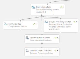
This set starts off with a Clean Missing Data tool. Let's see what it does.
 |
| Clean Missing Data (Left) |
As you can see, this tool takes all numeric columns, and substitutes 0 any time that the value is missing. The process of replacing missing values is called Imputation and it's a big deal in the data science world. You can read up on it
here. This tool also has the option to generate a missing value indicator column. This means that any row where a value was imputed would a value of 1 (or TRUE) and all other rows would have a value of 0 in the column. While we would love to go in-depth about imputation, it's a subject we'll have to reserve for a later post.
In our opinion, the coolest part about this tool has nothing to do with its goal. It has one of the best column selection interfaces we've ever seen. It allows you to programatically add or remove columns from your dataset. Looking at some of the other tools, this column selection interface pops in up in quite a few of them. This makes us very happy.
 |
| Select Columns |
We'll skip over the Summarize Data tool, as that was covered in the previous
post. Let's move on to the Evaluate Probability Function tool.
 |
| Evaluate Probability Function (Left) |
There are a couple of things to note about this tool. First, it lets you pick from a very large list of distributions.
 |
| Distributions |
It chose to use the Normal Distribution, which is what people are talking about when they say "Bell-Shaped Curve". It's definitely the most common used algorithm by beginner data scientists. Next, it lets you select which method you would like to use.
 |
| Method |
There are three primary methods in statistics, the Probability Density Function (PDF), Cumulative Distribution Function (CDF), and Inverse Cumulative Distribution Function (Inverse CDF). If you want to look these up on your own, you can use the following links:
PDF,
CDF,
InverseCDF.
You can get entire degrees just by learning these three concepts and we won't even attempt to explain them in a sentence. Simply put, if you want to see how likely (or unlikely) an observation is, use the CDF. We'll leave the other two for you to research on your own. Let's move on to the Select Columns tool.
 |
| Select Columns (Left) |
This tool is about as simple as it comes. You tell it which columns you want (using that awesome column selector) and it throws the rest away. Let's move on to the final tool, Compute Linear Correlation.
 |
| Compute Linear Correlation (Left) |
This is another simple tool. You give it a data set with a bunch of numeric columns, it spits out a matrix of Pearson correlations.
 |
| Linear (Pearson) Correlations (Left) |
These are the traditional correlations you learned back in high school. A correlation of 0 means that there is no linear relationship and a correlation of 1 or -1 means there is a perfect linear correlation.
We were planning on moving on to the other legs of this experiment. However, they are just slightly altered versions of what we went through. This is an interesting sample for Microsoft to publish, as it doesn't seem to have any real analytical value. We can't imagine using this is any sort of investigative or analytic scenario. What is it good for then? Learning Azure ML! This is exactly what we used it for. It showed us some neat features and prompted a few good follow-up posts to get more in-depth on some of these tools. Hopefully, it sparked some good ideas in you guys too. Thanks for reading. We hope you found this informative.
Brad Llewellyn
BI Engineer
Valorem Consulting
@BreakingBI
www.linkedin.com/in/bradllewellyn
llewellyn.wb@gmail.com


No comments:
Post a Comment