Azure Machine Learning in Practice: Productionalization

Today, we're going to finish up our Fraud Detection experiment.  If you haven't read our previous posts in this series, it's recommended that you do so.  They cover the Preparation, Data Cleansing, Model Selection, Model Evaluation, Threshold Selection, Feature Selection and Feature Engineering phases of the experiment.  In this post, we're going to walk through the Productionalization process.

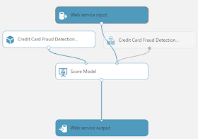
Productionalization is the process of taking the work we've done so far and making it accessible to the end user.  This is by far the most important process.  If we are unable to connect the end user to the model, then everything up until now was for nothing.  Fortunately, this is where Azure Machine Learning really differentiates itself from the rest of the data science tools on the market.  First, let's create a simple experiment that takes our testing data and scores that data using our trained model.  Remember that we investigated the use of some basic engineered features, but found that they didn't add value.

Productionalization

Now, let's take a minute to talk about web services.  A web service is a simple resource that sits on the Internet.  A user or application can send a set of data to this web service and receive a set of data in return, assuming they have the permissions to do so.  In our case, Azure Machine Learning makes it incredibly simple to create a deploy our experiement as an Azure Web Service.

Set Up Web Service

On the bar at the bottom of the Azure Machine Learning Studio, there's a button for "Set Up Web Service".  If we click it, we get a neat animation and a few changes to our experiment.

Predictive Experiment

We can see that we now have two new modules, "Web Service Input" and "Web Service Output".  When the user or application hits the web service, these are what they interact with.  The user or application passes a data set to the web service as a JSON payload.  Then, that payload flows into our Predictive Experiment and is scored using our model.  Finally, that scored data set is passed back to the user or application as a JSON payload.  The simplicity and flexibility of this type of model means that virtually any environment can easily integrate with Azure Machine Learning experiments.  However, we need to deploy it first.

Deploy Web Service

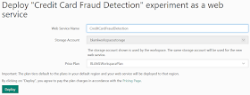
Just like with creating the web service, deployment is as easy as clicking a button on the bottom bar.  Unless you have a reason, it's good practice to deploy a new web service, as opposed to a classic one.

Web Service Deployment

Now, all we have to do is link it to a web service plan and we're off!  You can find out more about web service plans and their pricing here.  Basically, you can pay-as-you-go or you can buy a bundle at a discount and pay for any overges.  Now, let's take a look at a brand new portal, the Azure Machine Learning Web Services Portal.

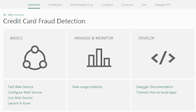
Azure Machine Learning Web Services Portal

This is where we can manage and monitor all of of our Azure Machine Learning Web Services.  We'll gloss over this for now, as it's not the subject of this post.  However, we may venture back in a later post.  Let's move over to the "Consume" tab.

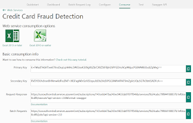
Azure Machine Learning Web Service Consumption Information

On this tab, we can find the keys and URIs for our new web services.  However, there's something far more powerful lurking further down on the page.

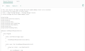
Sample Web Service Code

Azure Machine Learning provides sample code for calling the web service using four languages, C#, Python, Python 3+ and R.  This is amazing for us because we're not developers.  We couldn't code our way out of a box.  But, Azure Machine Learning makes it so easy that we don't have to.

Hopefully, this post sparked your imagination for all the ways that you could utilize Azure Machine Learning in your organization.  Azure Machine Learning is one of the best data science tools on the market because it drastically slashes the amount of time it takes to build, evaluate and productionalize your machine learning algorithms.  Thanks for reading.  We hope you found this informative.

Brad Llewellyn
Data Science Consultant
Valorem
@BreakingBI
www.linkedin.com/in/bradllewellyn
llewellyn.wb@gmail.com

Azure Machine Learning in Practice: Feature Selection

Today, we're going to continue with our Fraud Detection experiment.  If you haven't read our previous posts in this series, it's recommended that you do so.  They cover the Preparation, Data Cleansing, Model Selection, Model Evaluation and Threshold Selection phases of the experiment.  In this post, we're going to walk through the feature selection process.

In the traditional data science space, feature selection is generally one of the first phases of a modelling process.  A large reason for this is that, historically, building models using a hundred features would take a long time.  Also, an individual would have to sort through all of the features after modeling to determine what impact the features were having.  Sometimes, they would even find that some features would make the model less accurate by including them.  There's also the concept of parsimony to consider.  Basically, less variables was generally considered better.

However, technology and modelling techniques have come a long way over the last few decades.  We would be doing a great disservice to modern Machine Learning to say that it resembles traditional statistics in a major way.  Therefore, we try to approach feature selection from a more practical perspective.

First, we found that we were able to train over 1000 models in about an hour and a half.  Therefore, removing features for performance reasons is not necessary.  However, in other cases, it may be.  In those cases, paring down features initially could be beneficial.

Now, we need to determine which variables are having no (or even negative) impact on the resulting model.  If they aren't helping, then we should remove them.  To do this, we can use a technique known as Permutation Feature Importance.  Azure Machine Learning even has a built-in module for this.  Let's take a look.

Feature Selection Experiment

Permutation Feature Importance

This module requires us to input our trained model, as well as a testing dataset.  We also have to decide which metric we would like to use.  With that, it will output a dataset showing us the impact that each feature has on the model.

So, how does Permutation Feature Importance work?  Honestly, it's one of more clever algorithms we've come across.  The module chooses one feature at a time, randomly shuffles the values for that feature across the different rows, then retrains the model.  Then, it can evaluate the impact of that feature by seeing how much the trained model changed when the values were shuffled.  A very important feature would obviously cause large changes in the model if they were shuffled.  A less important feature would have less impact.  In our case, we want to measure impact by using Precision and Recall.  Unfortunately, the module only gives us the option to use one at a time.  Therefore, we'll have to be more creative.  Let's start by looking at the output of the Precision module.

Feature Importance (Precision) 1

Feature Importance (Precision) 2

We can see that there a few features that are important.  The rest of the features have no impact on the model.  Let's look at the output from the Recall module.

Feature Importance (Recall) 1

Feature Importance (Recall) 2

Now, let's compare the results of the two modules.

Feature Importance

We can see that the two modules have almost the same output, except for V4, which is only important for Precision.  This means that we should be able to remove all of the other features without affecting the model.  Let's try it and see what happens.

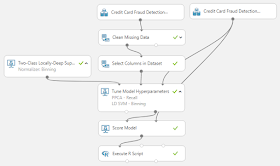
Feature Reduction Experiment

Tune Model Hyperparameters Results

R Script Results

We can see that removing those features from the model did reduce the Precision and Recall.  There was not a dramatic reduction in these values, but there was a reduction nonetheless.  This is likely caused by rounding error.  What was originally a very small decimal value assigned to the importance of each feature was rounded to 0, causing us to think that there was no importance.  Therefore, we are at a decision point.  Do we remove the features knowing that they slightly hurt the model?  Since we're having no performance issues and model understandability is not a factor, we would say no.  It's better to keep the original model than it is to make a slimmer version.

It is important to note that in practice, we've never seen the "Permutation Feature Importance" model throw out the majority of the features.  Usually, there are a few features that have a negative impact.  As we slowly remove them one at a time, we eventually find that most of the features have a positive impact on the model.  While we won't get into the math behind the scenes, we will say that we highly suspect this unusual case was caused by the fact that we are only given a subset of the Principal Components created using Principal Components Analysis.

Hopefully, this post enlightened you to some of the thought process behind Feature Selection in Azure Machine Learning.  Permutation Feature Importance is a fast, simple way to improve the accuracy and performance of your model.  Stay tuned for the next post where we'll be talking about Feature Engineering.  Thanks for reading.  We hope you found this informative.

Brad Llewellyn
Data Scientist
Valorem
@BreakingBI
www.linkedin.com/in/bradllewellyn
llewellyn.wb@gmail.com

Azure Machine Learning in Practice: Threshold Selection

Today, we're going to continue with our Fraud Detection experiment.  If you haven't read our previous posts in this series, it's recommended that you do so.  They cover the Preparation, Data Cleansing, Model Selection and Model Evaluation phases of the experiment.  In this post, we're going to walk through the threshold selection process.

So far in this experiment, we've taken the standard Azure Machine Learning evaluation metrics without much thought.  However, an important thing to note is that all of these evaluation metrics assume that the prediction should be positive when the predicted is probability is greater than .5 (or 50%), and negative otherwise.  This doesn't have to be the case.

In order to optimize the threshold for our data, we need a data set, a model and a module that optimizes the threshold for the data set and model.  We already have a data set and a model, as we've spent the last few post building those.  What we're missing is a module to optimize the threshold.  For this, we're going to use an Execute R Script.

Execute R Script

Execute R Script Properties

We talked about R scripts in one of our very first Azure Machine Learning posts.  This is one of the ways in which Azure Machine Learning allows us to expand its functionality.  Since Azure Machine Learning doesn't have the threshold selection capabilities we're looking for, we'll build them ourselves.  Take a look at this R Script.

CODE BEGIN

dat <- maml.mapInputPort(1)

###############################################################
## Actual Values must be 0 for negative, 1 for positive.
## String Values are not allowed.
##
## You must supply the names of the Actual Value and Predicted
## Probability columns in the name.act and name.pred variables.
##
## In order to hone in on an optimal threshold, alter the
## values for min.out and max.out.
##
## If the script takes longer than a few minutes to run and the
## results are blank, reduce the num.thresh value.
###############################################################

name.act <- "Class"
name.pred <- "Scored Probabilities"
name.value <- c("Scored Probabilities")
num.thresh <- 1000
thresh.override <- c()
num.out <- 20
min.out <- -Inf
max.out <- Inf
num.obs <- length(dat[,1])
cost.tp.base <- 0
cost.tn.base <- 0
cost.fp.base <- 0
cost.fn.base <- 0

#############################################
## Choose an Optimize By option.  Options are
## "totalcost", "precision", "recall" and
## "precisionxrecall".
#############################################

opt.by <- "precisionxrecall"

act <- dat[,name.act]
act[is.na(act)] <- 0
pred <- dat[,name.pred]
pred[is.na(pred)] <- 0
value <- -dat[,name.value]
value[is.na(value)] <- 0

#########################
## Thresholds are Defined
#########################

if( length(thresh.override) > 0 ){
thresh <- thresh.override
num.thresh <- length(thresh)
}else if( num.obs <= num.thresh ){
thresh <- sort(pred)
num.thresh <- length(thresh)
}else{
thresh <- sort(pred)[floor(1:num.thresh * num.obs / num.thresh)]
}

#######################################
## Precision/Recall Curve is Calculated
#######################################

prec <- c()
rec <- c()
true.pos <- c()
true.neg <- c()
false.pos <- c()
false.neg <- c()
act.true <- sum(act)
cost.tp <- c()
cost.tn <- c()
cost.fp <- c()
cost.fn <- c()
cost <- c()

for(i in 1:num.thresh){
thresh.temp <- thresh[i]
pred.temp <- as.numeric(pred >= thresh.temp)
true.pos.temp <- act * pred.temp
true.pos[i] <- sum(true.pos.temp)
true.neg.temp <- (1-act) * (1-pred.temp)
true.neg[i] <- sum(true.neg.temp)
false.pos.temp <- (1-act) * pred.temp
false.pos[i] <- sum(false.pos.temp)
false.neg.temp <- act * (1-pred.temp)
false.neg[i] <- sum(false.neg.temp)
pred.true <- sum(pred.temp)
prec[i] <- true.pos[i] / pred.true
rec[i] <- true.pos[i] / act.true
cost.tp[i] <- cost.tp.base * true.pos[i]
cost.tn[i] <- cost.tn.base * true.neg[i]
cost.fp[i] <- cost.fp.base * false.pos[i]
cost.fn[i] <- cost.fn.base * false.neg[i]
}

cost <- cost.tp + cost.tn + cost.fp + cost.fn
prec.ord <- prec[order(rec)]
rec.ord <- rec[order(rec)]

plot(rec.ord, prec.ord, type = "l", main = "Precision/Recall Curve", xlab = "Recall", ylab = "Precision")

######################################################
## Area Under the Precision/Recall Curve is Calculated
######################################################

auc <- c()

for(i in 1:(num.thresh - 1)){
                auc[i] <- prec.ord[i] * ( rec.ord[i + 1] - rec.ord[i] )
}

#################
## Data is Output
#################

thresh.out <- 1:num.thresh * as.numeric(thresh >= min.out) * as.numeric(thresh <= max.out)
num.thresh.out <- length(thresh.out[thresh.out > 0])
min.thresh.out <- min(thresh.out[thresh.out > 0])

if( opt.by == "totalcost" ){
opt.val <- cost
}else if( opt.by == "precision" ){
opt.val <- prec
}else if( opt.by == "recall" ){
opt.val <- rec
}else if( opt.by == "precisionxrecall" ){
opt.val <- prec * rec
}

ind.opt <- order(opt.val, decreasing = TRUE)[1]

ind.out <- min.thresh.out + floor(1:num.out * num.thresh.out / num.out) - 1
out <- data.frame(rev(thresh[ind.out]), rev(true.pos[ind.out]), rev(true.neg[ind.out]), rev(false.pos[ind.out]), rev(false.neg[ind.out]), rev(prec[ind.out]), rev(rec[ind.out]), rev(c(0, auc)[ind.out]), rev(cost.tp[ind.out]), rev(cost.tn[ind.out]), rev(cost.fp[ind.out]), rev(cost.fn[ind.out]), rev(cost[ind.out]), rev(c(0,cumsum(auc))[ind.out]), thresh[ind.opt], prec[ind.opt], rec[ind.opt], cost.tp[ind.opt], cost.tn[ind.opt], cost.fp[ind.opt], cost.fn[ind.opt], cost[ind.opt])
names(out) <- c("Threshold", "True Positives", "True Negatives", "False Positives", "False Negatives", "Precision", "Recall", "Area Under P/R Curve", "True Positive Cost", "True Negative Cost", "False Positive Cost", "False Negative Cost", "Total Cost", "Cumulative Area Under P/R Curve", "Optimal Threshold", "Optimal Precision", "Optimal Recall", "Optimal True Positive Cost", "Optimal True Negative Cost", "Optimal False Positive Cost", "Optimal False Negative Cost", "Optimal Cost")

maml.mapOutputPort("out");

CODE END

We created this piece of code to help us examine the area under the Precision/Recall curve (AUC in Azure Machine Learning Studio refers to the area under the ROC curve) and to determine the optimal threshold for our data set.  It even allows us to input a custom cost function to determine how much money would have been saved and/or generated using the model.  Let's take a look at the results.

Experiment

Execute R Script Outputs

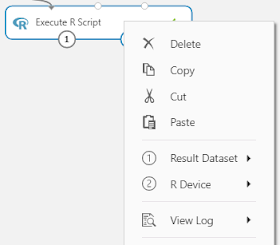
We can see that there are two different outputs from the "Execute R Script" module.  The first output, "Result Dataset", is where the data that we are trying to output is sent.  The second output, "R Device", is where any console displays or graphics are set.  Let's take a look at our results.

Execute R Script Results 1

Execute R Script Results 2

Execute R Script Graphics

We can see that this script outputs a subset of the thresholds evaluated, as well as the statistics using that threshold.  Also, it outputs the optimal threshold evaluated using a particular parameter that we will look at shortly.  Finally, it draws a graph of the Precision/Recall Curve.  For technical reasons, this graph is an approximation of the curve, not a complete representation.  A more accurate version of this curve can be seen in the "Evaluate Model" module.  We can choose our optimization value using the following set of code.

#############################################

## Choose an Optimize By option.  Options are

## "totalcost", "precision", "recall" and

## "precisionxrecall".

#############################################

opt.by <- "precisionxrecall"

In our case, we chose to optimize by using Precision * Recall.  Looking back at the results from our "Execute R Script", we see that our thresholds jump all the way from .000591 to .983291.  This is because the "Scored Probabilities" output from the "Score Model" module are very heavily skewed towards zero.  In turn, this skew is caused by the fact that our "Class" variable is heavily imbalanced.

Scored Probabilities Statistics

Scored Probabilities Histogram

Because of the way the R code is built, it determined that the optimal threshold of .001316 has a Precision of 82.9% and a Recall of 90.6%.  These values are worse than those originally reported by the "Tune Model Hyperparameters" module.  So, we can override the thresholds in our R code using the following code at the top of the batch:

thresh.override <- (10:90)/100

This will tell the R script to forcibly use thresholds from .10 to .90.  Let's check out the results.

Overridden Threshold Results 1

Overridden Threshold Results 2

We can see that by moving our threshold down to .42, we can tweak out slightly more value from our model.  However, this is a such a small amount of value that it's not worth any amount of effort to do it in this case.

So, when would this be useful?  As with everything, it all comes down to dollars.  We can talk to stakeholders and clients all day about how much Accuracy, Precision and Recall our models have.  In general, they aren't interested in that type of information.  However, if we can input an estimate of their cost function into this script, then we can tie real dollars to the model.  We were able to use this script to show a client that they could save $200k per year in lost product using their model.  That had far more impact than a Precision value ever would.

Hopefully, this post sparked your interest in tuning your Azure Machine Learning models to maximize their effectiveness.  We also want to emphasize that you can use R and Python to greatly extend the usefulness of Azure Machine Learning.  Stay tuned for the next post where we'll be talking about Feature Selection.  Thanks for reading.  We hope you found this informative.

Brad Llewellyn
Data Scientist
Valorem
@BreakingBI
www.linkedin.com/in/bradllewellyn
llewellyn.wb@gmail.com

Azure Machine Learning in Practice: Model Evaluation

Today, we're going to continue with our Fraud Detection experiment.  If you haven't read our previous posts in this series, it's recommended that you do so.  They cover the Preparation, Data Cleansing and Model Selection phases of the experiment.  In this post, we're going to walk through the model evaluation process.

Model evaluation is "where the rubber meets the road", as they say.  Up until now, we've been building a large list of candidate models.  This is where we finally choose the one that we will use.  Let's take a look at our experiment so far.

Experiment So Far

We can see that we have selected two candidate imputation techniques and fourteen candidate models.  However, the numbers are about get much larger.  Let's take a look at the workhorse of our experiment, "Tune Model Hyperparameters".

Tune Model Hyperparameters

We've looked at this module in some of our previous posts (here and here).  Basically, this module works by allowing us to define (or randomly choose) sets of hyperparameters for our models.  For instance, if we run the "Two-Class Boosted Decision Tree" model through this module with our training and testing data, we get an output that looks like this.

Sweep Results (Two-Class Boosted Decision Tree)

The result of the "Tune Model Hyperparameters" module is a list of hyperparameter sets for the input model.  In this case, it is a list of hyperparameters for the "Two-Class Boosted Decision Tree" model, along with various evaluation metrics.  Using this module, we can easily test tens, hundreds or even thousands of different sets of hyperparameters in order to find the absolute best set of hyperparameters for our data.

Now, we have a way to choose the best possible model.  The next step is to choose which evaluation metric we will use to rank all of these candidate models.  The "Tune Model Hyperparameters" module has a few options.

Evaluation Metrics

This is where a little bit of mathematical background can help tremendously.  Without going into too much detail, there's a problem with using some of these metrics on our dataset.  Let's look back at our "Class" variable. 

Class Statistics

Class Histogram

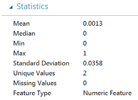
We see that the "Class" variable is extremely skewed, with 99.87% of all observations having a value of 0.  Therefore, traditional metrics such as Accuracy and AUC are not acceptable.  To further understand this, imagine if we built a model that always predicted 0.  That model would have an accuracy of 99.87%, despite being completely useless for our use case.  If you want to learn more, you can check out this whitepaper.  Now, we need to utilize a new set of metrics.  Let's talk about Precision and Recall.

Precision is the percentage of predicted "positive" records (Class = 1 -> "Fraud" in our case) that are correct.  Notice that we said PREDICTED.  Precision looks at the set of records where the model thinks Fraud has occurred.  This metric is calculated as

(Number of Correct Positive Predictions) / (Number of Positive Predictions)

One of the huge advantages of Precision is that it doesn't care how "rare" the positive case is.  This is extremely beneficial in our case because, in our opinion, 0.13% is extremely rare.  We can see that we want precision to be as close to 1 (or 100%) as possible.

On the other hand, Recall is the percentage of actual "positive" records that are correct.  This is slightly different from Precision in that it looks at the set of records where Fraud has actually occurred.  This metric is calculated as

(Number of Correct Positive Predictions) / (Number of Actual Positive Records)

Just as with Precision, Recall doesn't care how rare the positive case is.  Also like Precision, we want this value to be as close to 1 as possible.

In our minds, Precision is a measure of how accurate your fraud predictions are, while Recall is a measure of how much fraud the model is catching.  Let's look back at our evaluation metrics for the "Tune Model Hyperparameters" module.

Evaluation Metrics

We can see that Precision and Recall are both in this list.  So, which one do we choose?  Honestly, we don't have an answer for this.  So, we'll go back to our favorite method, try them both!

Model Evaluation Experiment

This is where Azure Machine Learning really provides value.  In about thirty minutes, we were able to set up this experiment that's going to create two evaluation metrics against fourteen sets of twenty models utilizing two cleansing techniques.  That's a total of 1,120 models!  After this finishes, we copy all of these results out to an Excel spreadsheet so we can take a look at them.

MICE - Precision - Averaged Perceptron Results

Our Excel document is simply a series of tables very similar to this one.  They show the parameters used for the model, as well as the evaluation statistics for that model.  Using this, we could easily find the combination of model, parameters and cleansing technique that gives us the highest Precision or Recall.  However, this still requires us to choose one or the other.  Looking back at the definitions of these metrics, they cover two different, important cases.  What if we want to maximize both?  Since we have the data in Excel, we can easily add a column for Precision * Recall and find the model that maximizes that value.

PPCA - Recall - LD SVM - Binning Results

As we can see from this table, the best model for this dataset is to clean the data using Probabilistic Principal Component Analysis, then model the data using a Locally-Deep Support Vector Machine with a Depth of 4, Lambda W of .065906, Lambda Theta Prime of .003308, Sigma of .106313 and 14,389 Iterations.  A very important consideration here is that we will not get the same results by copy-pasting these parameter values into the "Locally-Deep Support Vector Machine" module.  That's because these values are rounded.  Instead, we should save the best module directly to our Azure ML workspace.

Save Trained Model

At this point, we could easily consider this problem solved.  We have created a model that catches 90.2% of all fraud with a precision of 93.0%.  A very important point to note about this whole exercise is that we did not use domain knowledge, assumptions or "Rules of Thumb" to drive our model selection process.  Our model was selected entirely by using the data.  However,  there are a few more steps we can perform to tweak more power and performance out of our model.  Hopefully, this has opened your eyes to the Model Evaluation power of Azure Machine Learning.  Stay tuned for the next post where we'll discuss Threshold Selection.  Thanks for reading.  We hope you found this informative.

Brad Llewellyn
Data Scientist
Valorem
@BreakingBI
www.linkedin.com/in/bradllewellyn
llewellyn.wb@gmail.com

Azure Machine Learning in Practice: Model Selection

Today, we're going to continue with our Fraud Detection experiment.  If you haven't read our previous posts in this series, it's recommended that you do so.  They cover the Preparation and Data Cleansing phases of the experiment.  In this post, we're going to walk through the model selection process.

In traditional machine learning and data science applications, model selection is a time-consuming process that generally requires a significant amount of statistical background.  Azure Machine Learning completely breaks this paradigm.  As you will see in the next few posts, model selection is Azure Machine Learning requires nothing more than a basic understanding of the problem we are trying to solve and a willingness to let the data pick our model for us.  Let's take a look at our experiment so far.

Experiment So Far

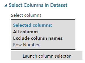
We can see that we've already imported our data and decided to use two different imputation methods, MICE and Probabilistic PCA.  Now, we need to select which models we would like to use to solve our problem.  It's important to remember that our goal is predict when a transaction is fraudulent, i.e. has a "Class" value of 1.  Before we do that, we should remember to remove the "Row Number" feature from our dataset, as it has no analytical value.

Select Columns in Dataset

Now, let's take a look at our model options.

Initialize Model

Using the toolbox on the left side of the Azure Machine Learning Studio, we can work our way down to the "Initialize Model" section.  Here, we have four different types of models, "Anomaly Detection", "Classification", "Clustering" and "Regression".

"Anomaly Detection" is the area of Machine Learning where we try to find things that look "abnormal".  This is an especially difficult task because it requires defining what's "normal".  Fortunately, Azure ML has some great tools that handle the hard work for us.  These types of models are very useful for Fraud Detection in areas like Credit Card and Online Retail transactions, as well Fault Detection in Manufacturing.  However, our training data already has fraudulent transactions labelled.  Therefore, Anomaly Detection may not be what we're looking for.  However, one of the great things about Data Science is that there are no right answers.  Feel free to add some Anomaly Detection algorithms to the mix if you would like.

"Classification" is the area of Machine Learning where we try to determine which class a record belongs to.  For instance, we can look at information about a person and attempt to determine where they are likely to buy a particular product.  This technique requires that we have an initial set of data where already know the classes.  This is the most commonly used type of algorithm and can be found in almost every subject area.  It's not coincidence that our variable of interest in this experiment is called "Class".  Since we already know whether each of these transactions was fraudulent or not, this is a prime candidate for a "Classification" algorithm.

"Clustering" is the area of Machine Learning where we try to group records together to identify which records are "similar".  This is a unique technique belonging to a category of algorithms known as "Unsupervised Learning" techniques.  They are unsupervised in the sense that we are not telling them what to look for.  Instead, we're simply unleashing the algorithm on a data set to see what patterns it can find.  This is extremely useful in Marketing where being able to identify "similar" people is important.  However, it's not very useful for our situation.

"Regression" is the area of Machine Learning where try to predict a numeric value by using other attributes related to it.  For instance, we can use "Regression" techniques to use information about a person to predict their salary.  "Regression" has quite a bit in common with "Classification".  In fact, there are quite a few algorithms that have variants for both "Classification" and "Regression".  However, our experiment only wants to predict a binary (1/0) variable.  Therefore, it would be inappropriate to use a "Regression" algorithm.

Now that we've decided "Classification" is the category we are looking for, let's see what algorithms are underneath it.

Classification

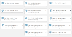
For the most part, we can see that there are two types of algorithms, "Two-Class" and "Multiclass".  Since the variable we are trying to predict ("Class") only has two values, we should use the "Two-Class" algorithms.  But which one?  This is the point where Azure Machine Learning really stands out from the pack.  Instead of choosing one, or even a few, algorithms, we can try them all.  In total, there are 9 different "Two-Class Classification" algorithms.  However, in the next post, we'll be looking at the "Tune Model Hyperparameters" module.  Using this module, we'll find out that there are actually 14 distinct algorithms, as some of the algorithms have a few different variations and one of the algorithms doesn't work with "Tune Model Hyperparameters".  Here's the complete view of all the algorithms.

Two-Class Classification Algorithms

For those that may have issues seeing the image, here's a list.

Two-Class Averaged Perceptron
Two-Class Boosted Decision Tree
Two-Class Decision Forest - Resampling: Replicate
Two-Class Decision Forest - Resampling: Bagging
Two-Class Decision Jungle - Resampling: Replicate
Two-Class Decision Jungle - Resampling: Bagging
Two-Class Locally-Deep Support Vector Machine - Normalizer: Binning
Two-Class Locally-Deep Support Vector Machine - Normalizer: Gaussian
Two-Class Locally-Deep Support Vector Machine - Normalizer: Min-Max
Two-Class Logistic Regression
Two-Class Neural Network - Normalizer: Binning
Two-Class Neural Network - Normalizer: Gaussian
Two-Class Neural Network - Normalizer: Min-Max
Two-Class Support Vector Machine

A keen observer may notice that the "Two-Class Bayes Point Machine" model was not included in this list.  For some reason, this model cannot used in conjunction with "Tune Model Hyperparameters".  However, we will handle this in a later post.

Hopefully, this post helped shed some light on "WHY" you would choose certain models over others.  We can't stress enough that the path to success is to let the data decide which model is best, not "rules-of-thumb" or theoretical guidelines.  Stay tuned for the next post, where we'll use large-scale model evaluation to pick the best possible model for our problem.  Thanks for reading.  We hope you found this informative.

Brad Llewellyn
Data Scientist
Valorem
@BreakingBI
www.linkedin.com/in/bradllewellyn
llewellyn.wb@gmail.com

Azure Machine Learning in Practice: Data Cleansing

Today, we're going to continue with our Fraud Detection experiment.  If you haven't read our previous post, it's highly recommended that you do, as it provides valuable context.  In this post, we're going to walk through the data cleansing process.

Data Cleansing is arguably one of the most important phases in the Machine Learning process.  There's an old programming adage "Garbage In, Garbage Out".  This applies to Machine Learning even more so.  The purpose of data cleansing is to ensure that the data we are using is "suitable" for the analysis we are doing.  "Suitable" is an amorphous term that takes on drastically different meanings based on the situation.  In our case, we are trying to accurately identify when a particular credit card purchase is fraudulent.  So, let's start by looking at our data again.

Credit Card Fraud Data 1

Credit Card Fraud Data 2

We can see that our data set is made up of a "Row Number" column, 30 numeric columns and a "Class" column.  For more information about what these columns mean and how they were created, read our previous post.  In our experiment, we want to create a model to predict when a particular transaction is fraudulent.  This is the same as predicting when the "Class" column equals 1.  Let's take a look at the "Class" column.

Class Statistics

Class Histogram

 Looking the histogram, we can see that we have heavily skewed data.  A simple math trick tells us that we can determine the Percentage of "1" values simply by looking at the mean times 100.  Therefore, we can see that 0.13% of our records are fraudulent.  This is what's known as an "imbalanced class".  An imbalanced class problem is especially tricky because we have to use a new set of evaluation metrics.  For instance, if we were to always guess that every record is not fraudulent, we would be correct 99.87% of the time.  While these seem like amazing odds, they are completely worthless for our analysis.  If you want to learn more, a quick google search brought up this interesting article that may be worth a read.  We'll touch on this more in a later post.  For now, let's keep this in the back of our mind and move on to summarizing our data.

Credit Card Fraud Summary 1

Credit Card Fraud Summary 2

Credit Card Fraud Summary 3

A few things stick out when we look at this.  First, all of the features except "Class" have missing values.  We need to take care of this.  Second, the "Class" features doesn't have missing values.  This is great!  Given that our goal is to predict fraud, it would be pretty pointless if some of our records didn't have a known value for "Class".  Finally, it's important to note that all of our variables are numeric.  Most machine learning algorithms cannot accept string values as input.  However, most of the Azure Machine Learning algorithms will transform any string features into numeric features.  You can find out more about Indicator Variables in an earlier post.  Alas, let's look at some of the ways to deal with our missing values.  Cue the "Clean Missing Data" module.

Clean Missing Data

The task of cleaning missing data is known as Imputation.  Given its importance, we've touched on it a couple of times on this blog (here and here).  The goal of imputation is to create a data set that gives us the "most accurate" answer possible.  That's a very vague concept.  However, we have a big advantage in that we have a data set with known "Class" values to test against.  Therefore, we can try a few different options to see which ones work best with our data and our models.

In the previous posts, we've focused on "Custom Substitution Value" just to save time.  However, our goal in this experiment is to create the most accurate model possible.  Given that goal, it would seem like a waste not to use some of more powerful tools in our toolbox.  We could use some of the simpler algorithms like Mean, Median or Mode.  However, we have a large number of dense features (this is a result of the Principal Component Analysis we talked about in the previous post).  This means that we have a perfect use case for the heavy-hitters in the toolbox, MICE and Probabilistic PCA (PPCA).  Whereas the Mean, Median and Mode algorithms determine a replacement value by utilizing a single column, the MICE and PPCA algorithm utilize the entire dataset.  This makes them extremely powerful at providing very accurate replacements for missing values.

So, which should we choose?  This is one of the many crossroads we will run across in this experiment; and the answer is always the same.  Let the data decide!  There's nothing stopping us from creating two streams in our experiment, one which uses MICE and one which uses PPCA.  If we were so inclined, we could create additional streams for the other substitution algorithms or a stream for no substitution at all.  Alas, that would greatly increase the development effort, without likely paying off in the end.  For now, we'll stick with MICE and PPCA.  Which one's better?  We won't know that until later in the experiment.

Hopefully, this post enlightened you to some of the ways that you can use Imputation and Data Cleansing to provide additional power to your models.  There was far more we could do here.  In fact, many data scientists approaching hard problems will spend most of their time adding new variables and transforming existing ones to create even more powerful models.  In our case, we don't like putting in the extra work until we know it's necessary.  Stay tuned for the next post where we'll talk about model selection.  Thanks for reading.  We hope you found this informative.

Brad Llewellyn
Data Scientist
Valorem
@BreakingBI
www.linkedin.com/in/bradllewellyn
llewellyn.wb@gmail.com