Monday, November 30, 2015

Level of Detail Calculations in Tableau Part 3: Distinct Counts

Today, we're going to talk about creating Distinct Counts in Tableau.  Primarily, we're going to focus on how to create them using Level of Detail (LoD) Calculations.  Then, we're going to compare LoDs to Table Calculations (TC) and Basic Calculations (BC) from the perspective of Ease of Creation, Flexibility and Performance.  We will not be covering in-depth how to create the Basic and Table Caclulation versions of the metrics.  COUNTD() is a built-in BC and you can read this post for the TC.  For these analyses, we will be using the Superstore Sales data set repeated 1000 times to create a data set that contains 10 million rows.

Metric 1: Total Distinct Rows

Let's start at the top level.  What if you wanted to know the Total Distinct Count of a field in your data set?
Distinct Rows (LoD)
Since we're looking for an overall Total, we want to use FIXED.  Our calculation in this case is COUNTD().  Let's check out the results.
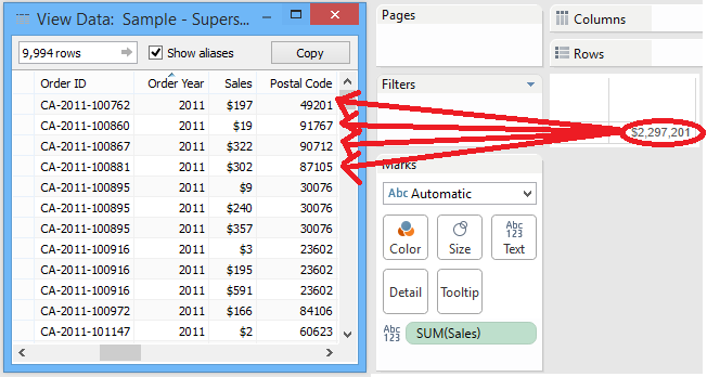
Total Distinct Rows (LoD)
We can see that we get one number and you can take our word for it that this number is correct.  Now, on to the interesting part.  How does this compare to using BC or TC?  BC would simply require us to use the COUNTD() with no FIXED wrapper, whereas a TC would require us to add the Row IDs to the canvas, then aggregate them out using another TC.  

From a ease of creation standpoint, BC is by far the simplest because COUNTD() is a built-in function.  LoD comes in second because it's the same calculation wrapped in a FIXED expression.  TC comes very far in last because it requires multiple TCs wrapped around some non-sensical functions (SUM() of a MAX() to be precise).

From a flexibility standpoint, BC and LoD tie for first.  BC would allow you to add any dimensions you want to the chart, but the value will change to represent what's in the chart.  On the other hand, adding a dimension to the chart would not change the LoD.  However, you could change the way you calculate your LoD in order account additional dimensions.  Again, TC come in last because adding a new dimension to the chart would probably require you to update your Compute Using in order to allow for accurate results.

Finally, let's look at the Performance Monitor.
Total Distinct Rows (PM)
As we can see, there was no performance difference between BC and LoD, whereas TC took almost 10 seconds to load this simple calculation.  This is an easy decision

VERDICT: BC if you want it to respond to added dimensions, LoD if you don't.

Metric 2: Distinct Customers that purchased at least 1 item over $100 by Category

This question is a little more difficult.  We have to be able to identify which items cost over $100.  Fortunately, our data is already at the item level.  So, this problem comes down to using a traditional filter.  We want to start by adding [Sales] to the filter shelf.  Not SUM( [Sales] ), just [Sales].  You can achieve this by right-click-dragging [Sales] to the filter shelf, and selecting "All Values" or you can drag [Sales] to the dimensions shelf, then to the filter shelf.  The choice is yours.  This filter will remove all rows from the underlying data that have a [Sales] value less than 100.  Now, there are two ways we can approach this, using INCLUDE/EXCLUDE or using FIXED.  Let's start with INCLUDE/EXCLUDE.
Distinct Customers (INCLUDE)
Distinct Customers with an item over $100 by Segment (INCLUDE)
We saw in Part 2 of this series that INCLUDE/EXCLUDE LoDs are calculated AFTER traditional filters.  Therefore, simply making this an INCLUDE/EXCLUDE LoD with no dimension allows it to be calculated after the filter.  Let's look at the FIXED version.

Distinct Customers (FIXED)
Distinct Customers with an item over $100 by Segment (FIXED) (incorrect)
Hmmm.  There's an issue here.  The numbers aren't the same as before.  Part 2 also mentioned that FIXED LoDs are calculated BEFORE traditional filters.  This means that this LoD sees ALL Customers, not just the ones we've filtered for.  We can alleviate this by adding the Sales filter to the Context (which is created before FIXED LoDs).
Distinct Customers with an item over $100 by Segment (FIXED)
Voila.  It works.  Now, let's consider the comparison.

From an ease of creation standpoint, BC wins again due to the fact that we're using a built-in calculation.  LoD runs in a close second, but does require some extra knowledge about order of operations in Tableau.  Finally, TC is just as unwieldy here as it was before.

The story is the same as last time from a flexibility standpoint.  It all depends on what your next step is.  If you want to continually add and remove dimensions to flow through your analysis, then BC is what you want.  However, if you want these totals to stay the same while you run simultaneous analyses, then a FIXED LoD is what you need.  We can't think of any reason why you would want to use an INCLUDE/EXCLUDE LoD in this situation instead of BC, but that doesn't mean there isn't one.  Lastly, TC suffers from the same issues it did on the first metric.  Compute Using is not going to be your friend in this case.

Let's check out the Performance.
Distinct Customers with an item over $100 by Segment (PM)
There doesn't seem to any discernable difference between most of the Calculation Types.  This is actually surprising because of how poorly TC performed in the first test.  It just goes to show that TCs can be very useful when there aren't a large number of marks on the chart.

VERDICT: BC if you want it to respond to added dimensions, FIXED LoD if you don't.

Metric 3: Distinct Customers who spent at least $100 in 2013 by Segment.

While this metric may seem very similar to the previous one, there is one major difference.  Our data is not at the Year level, it's at the Order Line level.  That means that the underlying data set cannot be used to identify a Customer who spent $100 in 2013.  This means that BC is completely off the table.  Our only options now are TC and LoD.  Let's try it out.
Distinct Customers who spent at $100 (INCLUDE)
Distinct Customers who spent at least $100 in 2013 by Segment (INCLUDE)
This is when LoDs start to begin causing headaches.  We can filter the chart down to 2013 to start.  Next, we need to identify which customers spent more than $100.  Finally, we need to typecast the Boolean (T/F) values to Numeric (1/0) values.  Then, we can add those up.  An interesting thing to note about this data set is that each Customer ID exists in only 1 segment.  This means that we can use FIXED to exploit this for some extra efficiency.
Distinct Customers who spent at $100 (FIXED)
Distinct Customers who spent at least $100 in 2013 by Segment (FIXED)
Adding the filter to context, and changing the word INCLUDE to FIXED does the trick.  If the relationship between Customer ID and Segment wasn't perfectly cascading, then we would also need to have Segment in our FIXED partition.  Now, let's take a look at the comparison.

From an ease of use standpoint, they feel pretty similar.  It more comes down to what you're comfortable with.  Personally, we're more comfortable with TC because that's what we're much more experienced with.  However, the more we work with LoDs, the more see their value.

From a flexibility standpoint, we'd have to say that the INCLUDE LoD wins out.  It allows you to add any dimension to the chart you would like and the calculation will still work.  However, if you were add another dimension, Category for instance, you will get double counting because a customer is likely to have purchased from more than one Category.

Finally, let's look at the performance monitor.
Distinct Customers who spent at least $100 in 2013 by Segment (PM)
Turns out that there was no performance difference between INCLUDE and FIXED.  This is likely due to the cascading relationship between the two.  However, there was a massive performance difference (more than 3x) between TC and LoD.  Given what we've seen so far, we're willing to bet that this gap would grow even more as the number of marks gets larger.

VERDICT: LoD because of a significant performance increase.

Throughout this post, we've seen that there are multiple ways to approach each type of problem.  As far as distinct counts go, it seems that you should use COUNTD() whenever you can.  If you can't, then LoD is probably the next best option.  Thanks for reading.  We hope you found this informative.

The workbook for this post can be found here.

Brad Llewellyn
Business Intelligence Consultant
llewellyn.wb@gmail.com
http://www.linkedin.com/in/bradllewellyn

Monday, November 16, 2015

Level of Detail Calculations in Tableau Part 2: Fixed, Include and Exclude

Today, we're going to explore the 3 types of Level of Detail (LoD) Calculations in Tableau.  They each have their own strengths and weaknesses.

LoD Type 1: FIXED

FIXED is arguably the simplest LoD to use in Tableau.  It calculates the same value, the same way regardless of the viz you put it in.  Let's see a simple example.  We start with a chart that shows Sales by Category and Sub-category.
Sales by Category and Sub-category
Let's try to append Total Sales onto this chart.  Total Sales is a fixed calculation because it doesn't care which fields are in the chart.  It wants ALL sales.  The syntax for an LoD is as follows:

{ (LoD Type) [Dimension1], [Dimension2], etc. : Metric }

Overall Total Sales
Sales and Overall Total Sales by Category and Sub-category
Since we want Overall Total Sales, our LoD Type is going to be FIXED, we don't have any dimensions, and our metric is SUM( [Sales] ).  As you can see, this is quite simple to write and works perfectly when you drag it on the chart.  If you read Part 1, you will remember that high-level aggregations like this are not affecting by the outside aggregation.  Therefore, changing the SUM() to a MAX() does not affect the value in the chart.  We'll touch more on that in a later post.
Sales and Overall Total Sales by Category and Sub-Category (with MAX())
LoD Type 2: INCLUDE

INCLUDE is a slightly more advanced type of LoD.  An Include LoD looks at all of the dimensions in your chart, and adds another dimension to the list.  For instance, let's look at Sales by Category.
Sales by Category
Now, what if we wanted to know the Sales for the largest Sub-category within each Category.  We can simply INCLUDE Sub-category to solve this.
Sales of Largest Sub-category
This calculation will take the Dimensions in the chart (Category) and combine with the included Dimensions (Sub-category) to create a table of SUM( [Sales] ) by Category and Sub-category.
Sales by Category and Sub-category (again)
Now, if we set the overlying aggregation to be MAX(), it will take the maximum Sub-category Sales within each Category.  This is what we see on our final chart.
Sales of Largest Sub-category by Category
A quick comparison to the LoD table confirms that our calculations are correct.
Sales by Category and Sub-category (with Largest Sub-categories highlighted)
An astute reader might note that this calculation could also have been done using

{FIXED [Category], [Sub-category]: SUM( [Sales] )}

This is correct.  In fact, most of the simple calculations can be done using a number of different calculations.  The real differences come when the calculations get more advanced.  But that's for a later post.

LoD Type 3: EXCLUDE

EXCLUDE works the exact opposite of INCLUDE.  It removes a dimension that currently exists in your viz.  For instance, let's start with a chart of Sales by Category and Sub-category.
Sales by Category and Sub-category (for the 3rd time)
We want to calculate the Total Sales within each Category.
Total Category Sales
Sales and Total Category Sales by Category and Sub-category
It should be noted that when you are using INCLUDE and EXCLUDE, the value of the LoD may change if you change your viz.  For instance, let's take Category out of the above chart.
Sales and Total Category Sales by Sub-category (or not)
Using EXCLUDE to remove Sub-category now leaves us with no dimensions, which causes the Total Category Sales to reflect Overall Total Sales instead.  For this reason, it's generally a good idea to accurately name your calculations.  For instance, "Total Category Sales" should be "Sales Excluding Sub-category".

The final key difference between these 3 LoD Types is how they interact with filters.  FIXED LoDs are designed to work independently of the chart.  Therefore, their values are not affected by traditional filters.  They see what the chart sees (also known as the context).  However, INCLUDE and EXCLUDE LoD's are designed to work in the confines of a single viz.  Therefore, they are affected by traditional filters.  This leaves us with the following order of calculation.

1) Data Source Filters
2) Context Filters
3) FIXED LoDs
4) Traditional Filters
5) INCLUDE and EXCLUDE LoDs

We still have a tremendous amount of room to explore the great new feature of Level of Detail Calculations.  Thanks for reading.  We hope you found this informative.

The workbook for this post can be found here.

P.S.

A couple users on the Tableau forums pointed me towards this graphic which I think tells the story perfectly.

Brad Llewellyn
Director, Consumer Sciences
Consumer Orbit
llewellyn.wb@gmail.com
http://www.linkedin.com/in/bradllewellyn

Monday, November 2, 2015

Level of Detail Calculations in Tableau Part 1: What are they?!?

Today, we're going to look at one of the newest additions to Tableau v9, Level of Detail (LoD) calculations.  For a long time, our vizzes have been constrained by only being able to look at one "level of detail" at a time.  What's a level of detail, you ask?  A level of detail, also called the "grain" or "level of aggregation" is what Tableau sees when it tries to build your chart.  For instance, let's say you want a simple chart, Sales over Time.  You see this
Sales by Year (Line Chart)
However, Tableau sees this
Sales by Year (Table)
Tableau looks at your data source, adds up the Sales for each Year, then uses that table to draw your viz.  The issue with this is approach comes when you want to ask more questions.  What if you want to compare the Sales for each Year to the overall total?  Since the invention of Tableau, we've had to use table calculations to do this.  Basically, the table calculation would require Tableau to build the Sales by Year table, then sum all of the values in that table to get the Overall Total.  Next, it would have to append that value back to the table just to create the viz.
Sales and Overall Total Sales
If that sounds like a big circle, it's because it is.  As many of you have seen, as this underlying table gets larger and the table calculation gets more and more complex, the table calculation can get quite slow.

This is where Level of Detail calculations come in.  We could accomplish this simple task by using a level of detail calculation as well.
Overall Total Sales (LoD)
Sales and Overall Total Sales by Year (TC and LoD)
As you can see, we simply tell Tableau to calculate the value and everything magically works.  The question is "What is Tableau doing to make this work?"
Appending Overall Total Sales to Underlying Data
We originally thought that Tableau dives into the underlying data, calculates the Total Overall Sales, then appends that value back to the underlying data.  However, that doesn't seem to be the case.  If you drag that field onto the chart, it calculates it using the ATTR() function.
ATTR()
This function looks at every row in the underlying data source.  If every row has the same value, it returns that value.  If not, it returns *.  Since the LoD was calculated across ALL rows, the value is going to be the same across all rows.  After all, there is only one total.  This leads us to a question, "What would happen if you changed that aggregation to SUM() instead of ATTR()?"
Sales and Overall Total Sales by Year (with SUM())
Surprisingly, it doesn't change.  Apparently, Tableau is taking that 1x1 table of Overall Total Sales, and appending it to the Sales by Year table.  As usual, we have another question, "How does this differ from Table Calculations?"  They both calculate values and append them to the Yearly table.  However, Table Calculations can only use values within the Yearly table.  This means that if you wanted to append Maximum Monthly Sales within that Year, you would not be able to use a Table Calculation because Month is not in the table.  However, LoDs can do that easily.
Order YearMonth
Maximum Monthly Sales
For some reason, Tableau will not let you use formula when you are defining the partition for your LoD.  So, we had to create a unique identifier for every month and year in a separate calculation.  Then, we simply tell Tableau to calculate the Sum( [Sales]) for each month and year, then take the MAX().
Sales and Maximum Monthly Sales by Year
As you can see, Tableau found the largest monthly sales for each year.  This situation differs from the one we saw previously because changing the aggregation does change the result.  With a little investigation, it seems that Tableau creates a separate table for the LoD calculation, and appends it the "best" way it can.  In the case of Overall Total Sales, the calculation was fixed on Year and Year was in the table.  So, it was able to append the Year value directly to the table.  However, in this case, Month is not in the table.  So, it takes the external LoD table containing on the Sales by Month, and rolls it up to the Year level based on the aggregation we give it (in this case MAX()).  The cool thing about LoDs is that they can also adapt to new dimensions being added to the chart.
Sales and Maximum Monthly Sales by Year and Quarter
We see that the Maximum Monthly Sales has updated to calculate by Year and Quarter, instead of by Year.  This is not unique to LoDs by any means.  An intelligently designed Table Calculation will do this as well.  However, let's ask the same question we asked before.  This is the Maximum value, what happens if we change MAX() to SUM()?  Will we still get the same answer?
Total Monthly Sales
Sales, Maximum and Total Monthly Sales by Year
Sadly, we do not get the same answer.  However, every time we asked a question, we got the answer we wanted.  This is very interesting an opens up a whole slew of questions.  What's happening behind the scenes to make this happen?  In situations where there is more than one approach, which one will perform the best or is the easiest to maintain?  What kinds of problems can LoDs solve that were previously unsolvable?  These are the kinds of questions we will look into throughout.  Please join us on our adventure as we explore this strange new option of Level of Detail Calculations.  Thanks for reading.  We hope you found this informative.

The workbook for this post can be found here.

Brad Llewellyn
Director, Consumer Sciences
Consumer Orbit
llewellyn.wb@gmail.com
http://www.linkedin.com/in/bradllewellyn