Sunday, March 24, 2013

Creating Table Calculations on Values outside of the Filter Range in Tableau

Today, we will talk about creating table calculations for values that are being filtered out of your view in Tableau.  A common scenario for this is as follows: "I want to see this month's sales as well as a 12-month rolling average for last year."  Let's naively put this is a chart.  As usual, we will use the Superstore Sales sample data set in Tableau.

Step 1:
  • Create a 12-Month Rolling Average
  • Create the following calculated field
12-Month Rolling Average
We will use this calculation throughout this post, so don't go deleting it or creating a new workbook.

Step 2:
  • Drag Month to Columns Shelf
  • Drag Sales and 12-Month Rolling Average to the Rows Shelf
  • Turn on Dual Axis and Synchronize the Axes
  • Turn Sales into bars and 12-Month Rolling Average into a line
  • Filter the year to be 2012
Naive Rolling Average
There are two very important things to notice about this "Rolling Average."  To start, the first value in the line is exactly the first month's sales.  Also, the line gets more and more stable as we progress in time.  This is because our rolling average doesn't consider any values outside of our filter.  The only value that is a true 12-month rolling average is the value for December.

We can fix this by exploiting the order in which operations are performed in Tableau.  We want our table calculations to be evaluated before the data is filtered on year.  We know that Tableau executes all table calculations simultaneously.  Therefore, if we can use a table calculation to filter on year, then we will force Tableau to evaluate our table calculations before it filters on year.  Let's do this.

Step 1:
  • Examine the structure of the graph without a date filter
Unfiltered graph
Using this graph, we want to hide the first 36 bars (months) and show the last 12 bars (months).  There are many ways to do this; we will use the INDEX() function because it seems to be the most intuitive in this situation.

Step 2:
  • Create the following calculated field
2012 Filter
Step 3:
  • Make "2012 Filter" Discrete
  • Filter "2012 Filter" to be 1
True Rolling Average
Notice that the line is much smoother the entire way across the graph, indicating that it is evaluated properly.  There is no simple answer to this problem when you encounter it in your work.  You must be able to create your own clever table calculation depending on how your data looks.  Remember, there are plenty of table calculations to help with this, such as FIRST(), LAST(), or even WINDOW_SUM().  Depending on your situation, you may even be able to use the Pages Shelf.  I hope you found this informative.  Thanks for reading.

EDIT:

Joe Mako commented with the more elegant method of using LOOKUP( MIN( YEAR( [Order Date] ) ), 0 ) instead of the index on the months.  This just goes to show that there are many different ways to handle this situation.  Many thanks to him and all of the readers.

Brad Llewellyn
Associate Consultant
Mariner, LLC
llewellyn.wb@gmail.com
https://www.linkedin.com/in/bradllewellyn

Thursday, March 21, 2013

Working with Window Calculations and TOTAL() in Tableau

Today, we will talk about Window Calculations and the TOTAL() function in Tableau.  Window Calculations allow you to implement a second level of aggregation on top of your basic aggregations, such as SUM() and COUNT().  This post is the ancestor to Working with Table Calculations in Tableau.  If you are not familiar with Table Calculation and "Compute Using", you should read that post first.  This is also the first post where I am using Tableau 8.0.  As usual, we will use the Superstore Sales sample data set in Tableau.

First, let's look at the TOTAL() function.  The TOTAL() function applies the underlying aggregation to the entire pane instead of each individual row.

Step 1:
  • Create a text table with two hierarchical dimensions on the rows
Sales by Sub-Category
Step 2:
  • Calculate the total sales across all categories
  • Calculate the total sales for each category
  • Create the following calculated fields
Category Total
Overall Total
Take care to notice what values are being summarized over.

Step 3:
  • Add these values to the table
Sales by Sub-Category (with Totals)
This example is somewhat silly because this is much better accomplished by adding Row Subtotals.  However, this is a great example to show how the TOTAL() function works.  

Now, let's move on to Window Calculations.  We will use WINDOW_SUM(); however, the same techniques can be applied for the other Window Calculations as well.  A Window Calculation requires three input parameters.  These parameters are an aggregated value, a displacement value for the starting point, and a displacement value for the ending point.  For example, 

WINDOW_SUM( SUM( [Sales] ), 0, 0 )

will calculate the SUM of SUM of [Sales] for the current row only, which is just the SUM of [Sales]; whereas

WINDOW_SUM( SUM( [Sales] ), FIRST(), LAST() ) or just WINDOW_SUM( SUM( [Sales] ) )

will calculate the SUM of SUM of [Sales] for the entire pane, which is identical to using

TOTAL( SUM( [Sales] ) ).

Step 1:
  • Create a text table
Sales by Sub-Category
Step 2:
  • Calculate the sum of each Sub-Category along with the previous and next Sub-Category
  • Create the following calculated field
Sum of Neighbors
Step 3:
  • Add this value to the table
Sales by Sub-Category (with Sum of Neighbors)
Now, you can see that each value is the Sum of [Sales] for this Sub-Category as well as the two neighboring Sub-Categories.  Care should be taken to avoid situations such as the first as last row, where there is no previous or next value, respectively.

There is so much more to be done here.  Try combining Window Calculations with different aggregrations, such as Sums of Averages, or try creating your own Percent of Total calculations.  I hope you found this informative.  Thanks for reading.

Brad Llewellyn
Associate Consultant
Mariner, LLC
llewellyn.wb@gmail.com
https://www.linkedin.com/in/bradllewellyn

Monday, March 18, 2013

Combining Types of Graphs (Multiple Mark Types) in Tableau

Today, we will look how to combine different types of graphs in Tableau.  Specifically, we will create a bar graph of monthly sales, with a line for the running average.  As usual, we will use the Superstore Sales sample data set in Tableau.

Step 1:
  • Filter your graph for the year "2012"
  • Drag "Month" to the column shelf
  • Drag "Sales" to the row shelf
Sales by Month
Step 2:
  • Calculate the running average of sales
  • Create the following calculated field
Running Average of Monthly Sales
Step 3:
  • Add the calculation to the Rows Shelf
  • In the Marks Card, click the triangle in the upper-right corner -> Select "Multiple Mark Types"
  • Click the Right Arrow that appeared until you get to "Running Average of Monthly Sales"
  • Change the Mark Type to "Line"
  • Right-click the "Running Average of Monthly Sales" pill and select "Dual Axis"
  • Right-click on the right axis and select "Synchronize Axis"
Sales by Month with Running Average
Voila!  Mission complete.  However, this was only the tip of the iceberg.  There's so much more to be done here.  Try use different graph types for truly brilliant designs.  I will leave you with a more advanced chart that shows Profit by Sub-Category along with a "Pareto" line.
Profit by Sub-Category with Pareto Line
I hope you found this informative.  Thanks for reading.

Brad Llewellyn
Associate Consultant
Mariner, LLC
llewellyn.wb@gmail.com
https://www.linkedin.com/in/bradllewellyn

Wednesday, March 6, 2013

Conducting a 2-sample Z Test in Tableau

Yesterday, we posted a blog about finding the median of a set of Likert Values.  This got us thinking that maybe basic statistics are possible in Tableau.  As it turns out, they are.  Today, we will look at how to conduct a 2-sample Z Test in Tableau.  A 2-population Z Test determines whether two samples from normally distributed populations have the same mean.  As usual, we used the Superstore Sales sample data set in Tableau.

EDIT:  This instance is definitely a case of "foot-in-mouth" syndrome.  Later in this post, I use the incorrect formula to calculate the P-value.  However, the rest of the procedure is valid, just not the P-value.  Even so, this is still a good example of showing the many uses of table calculations.  Enjoy!

Step 1:
  • Determine what two sets of data you would like to compare
For our example, we chose profits for 2011 and 2012, rolled up to the customer level.  We can see these distributions below.
Histograms
For those of who know how to look at normal histograms, you can probably see that these are VERY similar.  Therefore, we should expect our test to return a high P-value (> .05).

Step 2: 
  • Aggregate your data and divide it into your two samples.
  • Create the following calculated fields.
2011 Profit
2012 Profit
Step 3:
  • Find the means and standard deviations of your two sets.
  • Create the following calculated fields.
2011 Profit Sample Mean
2012 Profit Sample Mean
2011 Profit Standard Deviation
2012 Profit Standard Deviation
There are two important things to note here.  First, these are all window functions along [Customer].  This is because we already aggregated the data up to the [Customer] level, and Tableau only gives us one option for a secondary aggregation.  Second, a discerning reader might say, "You're using sample standard deviations!  Shouldn't these be t tests?"  The answer is a resounding, "Yes!"  However, to our knowledge, Tableau does not have access to the Gamma function (Google it if you care what it is.).  This makes it impossible to calculate a P-value.  So, we're stuck with a z test, which is almost identical given our large sample size.

Step 4:
  • Calculate your pooled standard deviation
  • Create the following calculated fields
2011 Customers
2012 Customers
Pooled Profit Standard Deviation
The first two calculated fields are distinct counts of the number of customers.  We exploited the "Compute Along" feature to simplify the calculation to a simple sum of ones.

Step 5:
  • Calculate the Z Score
  • Create the following calculated field
Z Score
Step 6:
  • Calculate the P-value
  • Create the following calculated field
P-value
As you can see, this is a two-sided P-value, you can make it one sided if you so choose.  However, now we can look at the final result.

EDIT:  I had a big DUH! moment earlier today.  The formula I used to calculate the p-value is incorrect.  It should be an integral, which Tableau is incapable of calculating.  In spite of this, the Z-statistic is still valid, you just have to use some other means to calculate a rejection region and/or a P-value.  On the bright side, maybe some type of statistical package integration is in the works.  Cheers!

Final Table
The one caveat is that you have to put [Customer] somewhere in the canvas in order for this method to work.  We thought the level of detail would be the easiest.  As we suspected, the P-value is extremely high, meaning that we don't have enough evidence that say that these two samples come from populations with different means.

WHEW!  Wasn't that a lot of work?  We think so too.  It seems that we've shown that Tableau is capable of  basic statistical testing.  However, you are literally doing all of the work from scratch.  It would probably be much easier to combine Tableau's graphical capabilities with a more specialized tool, such as R or SAS.  On the bright side, there's an idea on the Tableau forums to put some sort of R integration in Tableau.  Here's to hoping!

In all seriousness though, if you need advanced statistical procedures, you're probably better off using a specialized tool and exporting the values manually.  I hope you found this informative.  Thanks for reading.

Brad Llewellyn
Associate Consultant
Mariner, LLC
llewellyn.wb@gmail.com
https://www.linkedin.com/in/bradllewellyn

Tuesday, March 5, 2013

Calculating the Median of a Likert (Survey) Scale in Tableau

Today, we will look at how to calculate the "median" of Likert Scale in Tableau.  Median is in quotes because this is not a true median, it is more like a weighted average.  However, I believe it gives you far more information than a true median and, therefore, is worth pursuing.  For those of you who are not familiar with a Likert Scale, it is as follows:

1 - Strongly Disagree
2 - Disagree
3 - Neither Agree nor Disagree
4 - Agree
5 - Strongly Agree

This is the common 5-point version; however, there are adaptations of 6 and 7 points as well.  On the bright side, the algorithm in this post will work for any number of points with no alterations.  For the first time, I had to create my own data set for this post.  The sets are as follows:

Sample Data
This idea is courtesy of a poster on the Tableau Forums, Stuart Ramsbottom. (If he gives me a better way to credit him, I will add it here.)  His original post on the Tableau forums can be found HERE.  Set 1 is actually his set of data, while Set 2 is a set I made up to test the algorithm.

Step 1:
  • The median record is found as a traditional median, i.e. Total Number of Records / 2.
  • Create the following calculated field
Median Record
Median Record Test
Step 2:
  • Find the upper threshold for each Likert Category, i.e. Calculate the Cumulative Number of Records.
  • Create the following calculated field
Cumulative Number of Records

Cumulative Number of Records Test
Step 3:
  • Using these upper thresholds, find the Likert Category corresponding the Median Record, i.e. < Threshold( Likert Category - 1 ) < Median Record <= Threshold( Likert Category ).
To me, this seems to be a difficult concept to communicate.  To put it more simply, you must find the Likert Category that the Median Record falls in.


  • Create the following calculated field
Median Likert Category
Median Likert Category Test
Step 4:
  • Find how "far" into the Likert Category the Median Record is, i.e. (Median Record - Lower Threshold of Likert Category) / Number of Records in this Likert Category
  • Create the following calculated field
Number of Values into Likert Category
Number of Values into Likert Category Test
Step 5:
  • Find the starting value of the Likert Category, i.e. the average of Likert Category and Likert Category - 1 = Likert Category - .5
  • Create the following calculated field
Start of Likert Category
Start of Likert Category Test
Step 6:
  • Take the Starting Value of the Median Likert Category, add the Number of Values into the Likert Category, i.e. Starting Value of Category + Number of Values into Category.
  • Apply this calculation only to the Median Likert Category (It is incorrect for every other category)
  • Create the following calculated field
Median Likert Score
Now, we can use see the final result of our work, the "Median" Likert Score for our data.
Final Result
We hope you found this informative.  Thanks for reading.

Brad Llewellyn
Associate Consultant
Mariner, LLC
llewellyn.wb@gmail.com
https://www.linkedin.com/in/bradllewellyn

Monday, March 4, 2013

Basic Function Types in Tableau

Today, we will talk about the different basic functions in Tableau.  This was prompted by a poster on the Tableau forums asking for more information about these functions.  I am not an expert on Tableau's data engine.  Therefore, I will keep this discussion somewhat high-level.

SQL FUNCTIONS

These functions all exist in the SQL language.  It is my hypothesis that they are passed directly to the underlying SQL for computational efficiency.  However, this is one area I am currently looking into.  If anyone knows for sure, please let me know in the comments.

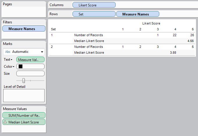
COUNT( [Any Row-Level Data Type] )

This function returns the number of non-null rows in the pane.  If you have a complete data set, this will be identical to SUM( 1 ).  This function is useful if you want to know how many rows satisfy a certain condition.  For example, you can find the number of rows from 2013 with

     IF [Year] = 2013 THEN COUNT( [Year] ) END

SUM( [Row-Level Numeric] )

This function returns the sum of non-null rows in the pane.  I believe it to be the easiest function to comprehend.  For example, you can find total sales with

     SUM( [Sales] )

AVG( [Row-Level Numeric] )

This function returns the average of non-null rows in the pane.  Care should be taken when working with this function.  It returns the sum of all non-null rows divided by the count of all non-null rows.  If you want an average calculated at a level that isn't the row-level, you need to create your own SUM() and COUNT() functions.  For example, you can find average profit with

     AVG( [Profit] )

COUNTD( [Any Row-Level Data Type] )

This function returns the distinct count of non-null rows in the pane.  It is especially useful for calculating averages at a different grain than your underlying data.  If my data was at the transaction level, I could calculate the average profit per store as

     SUM( [Profit] ) / COUNTD( [StoreNumber] )

DATEADD( [Date Unit], [Integer], [Date] )

This function adds a certain number of units to a date value.  The unit type and number of units are supplied by the user.  For example, 3 days after [Date] can be found as

     DATEADD( "day", 3, [Date] )

DATEDIFF( [Date Unit], [Start Date], [End Date] )

This function returns the number of date units between the start and end dates.  For example, the number of years between [Date1] and [Date2] is

     DATEDIFF( "year", [Date1], [Date2] )

LEN( [String] )

This function returns the number of characters in a string.  For example, the number of characters in "Tableau" ( 7 ) is

     LEN( "Tableau" )

LEFT( [String], [Integer] )

This function returns the first [Integer] characters in a string.  For example, the first 4 characters in "Tableau" (Tabl) is

     LEFT( "Tableau", 4 )

TABLEAU FUNCTIONS

To my knowledge, these functions do not have direct relationships to SQL functions.  Therefore, my hypothesis is that these are calculated within Tableau.  If there is more to this, please let me know in the comments.

LOOKUP( [Function], [Offset] )

This is the workhorse of all window functions.  It returns the value of the given function at another value outside of the current pane.  This requires use of "Compute Using."  If you are not familiar with "Compute Using", please refer to my previous post Working with Table Calculations in Tableau.  For example, if you want to the see the value of SUM( [Sales] ) in the previous row, you can use

     LOOKUP( SUM( [Sales] ), -1 )

RUNNING_SUM( [Function] )

This function returns the sum of the function in all previous rows in the table.  For example, the sum of all previous daily counts is

     RUNNING_SUM( COUNT( [Sales] ) )

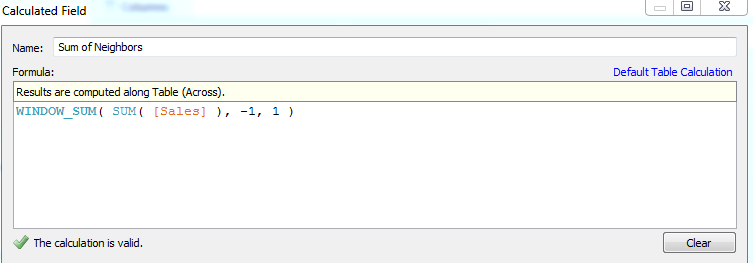
WINDOW_SUM( [Function], { [StartOffset], [EndOffset] } )

This function returns the sum of the function for all rows within the window defined by [StartOffset] and [EndOffset].  This is the first occurrence of optional parameters.  If [StartOffset] and [EndOffset] are omitted, the entire table is used.  For example, if you would like to the sum of sales for the last 3 rows (4 rows total including the current row), you can use

     WINDOW_SUM( SUM( [Sales] ), -3, 0 )

FIRST()

This function returns the current offset from the first row.  For example, if you want to emulate RUNNING_SUM using WINDOW_SUM, you can use

     WINDOW_SUM( SUM( [Sales] ), FIRST(), 0 )

These are a good portion of the Tableau functions that I regularly use.  However, there are quite a few useful functions that are not mentioned here.  If you feel like I missed something important, let me know.  I hope you found this informative.  Thanks for reading.

Brad Llewellyn
Associate Consultant
Mariner, LLC
llewellyn.wb@gmail.com
https://www.linkedin.com/in/bradllewellyn